Dot Product

note

In the following text, we will abbreviate the dot product of a vector with itself using exponent notation, i.e.

$$\vec{v}^2 \coloneqq \vec{v} \cdot \vec{v}$$

Introduction

The dot-product takes two vectors and returns the sum of the component-wise products of the vector's components. Given two vectors

$$\vec{a}, \vec {b} \in \mathbb{R}^n, \vec{a} = \begin{pmatrix} a_1 \\ a_2 \\ \vdots \\ a_{n} \end{pmatrix}, \vec{b} = \begin{pmatrix} b_1 \\ b_2 \\ \vdots \\ b_{n} \end{pmatrix}$$

the dot product yields a scalar value.

$$\vec{a} \boldsymbol{\cdot} \vec{b} = \sum_{i=1}^{n} a_ib_i$$

Geometric Interpretation

If $\vec{a} \boldsymbol{\cdot} \vec{b} = 0$, the two vectors are perpendicular to each other. We will derive this in the following.

Orthogonality of Unit Vectors

We will first have a look at a special case, namely when $\vec{a}, \vec{b}$ are both unit vectors.

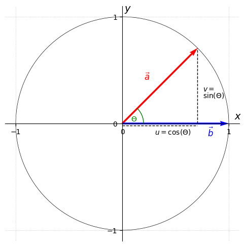
In Figure 1, the radius of the unit circle is represented by the vectors $\vec{a}$ and $\vec{b}$. Thus, for both $\vec{a}$ and $\vec{b}$ the following trivially holds:

$$|\vec{a}| = 1 \\ |\vec{b}| = 1$$

^{Figure 1 Unit Circle with two vectors a and b, which both have a magnitude of 1}

Plot-Code (Python)

import matplotlib.pyplot as plt
import numpy as np
from matplotlib.patches import Arc

fig, ax = plt.subplots(figsize=(6, 6))

# Plot setup
ax.set_xlim(-1.1, 1.1)
ax.set_ylim(-1.1, 1.1)
ax.set_xticks([-1, 0, 1])
ax.set_yticks([-1, 0, 1])
ax.set_aspect('equal')
ax.grid(True, linestyle=':', linewidth=0.5)

for spine in ax.spines.values():
    spine.set_visible(False)

ax.spines['bottom'].set_position('zero')
ax.spines['left'].set_position('zero')
ax.spines['bottom'].set_visible(True)
ax.spines['left'].set_visible(True)

ax.xaxis.set_ticks_position('bottom')
ax.yaxis.set_ticks_position('left')

ax.text(1.05, 0.02, r"$x$", fontsize=14, va='bottom')
ax.text(0.02, 1.05, r"$y$", fontsize=14, ha='left')

# Vecors
origin = np.array([0, 0])
theta = np.radians(45)
cos_theta = np.cos(theta)
sin_theta = np.sin(theta)
opposite = np.array([0, np.sin(theta)])
v1 = np.array([np.cos(theta), np.sin(theta)])
v2 = np.array([1, 0])

ax.quiver(*origin, *v1, angles='xy', scale_units='xy', scale=1, color='r')
ax.quiver(*origin, *v2, angles='xy', scale_units='xy', scale=1, color='b')

offset = 0.01
ax.text(v1[0] - 0.5, v1[1] -0.3, r"$\vec{a}$", fontsize=12, color='r')
ax.text(v2[0] - 0.2, v2[1]  -0.12, r"$\vec{b}$", fontsize=12, color='b')

# COSINE
ax.plot([0, cos_theta], [-0.02, -0.02], color='black', linestyle='--', linewidth=1)
ax.text(cos_theta / 2 - 0.05, -0.1, r"$\cos(\Theta)$", fontsize=10)

# SINE
start = np.array([cos_theta, 0])
end = start + opposite
ax.plot([start[0], end[0]], [start[1], end[1]], color='black', linewidth=1, linestyle='--')
ax.text(cos_theta + 0.05, sin_theta / 2 - 0.05, r"$\sin(\Theta)$", fontsize=10)


# Unit Circle
circle = plt.Circle((0, 0), 1, color='black', linewidth=0.5, fill=False, transform=ax.transData)
ax.add_patch(circle)

# Angle Arc
angle_deg = np.degrees(np.arccos(np.dot(v1, v2)))
arc = Arc(origin, 0.4, 0.4, angle=0, theta1=0, theta2=angle_deg, edgecolor='green')
ax.add_patch(arc)
ax.text(0.08, 0.02, r"$\Theta$", color='green')

plt.show()

Clearly, $\vec{b} = \begin{pmatrix} 1 \\ 0 \end{pmatrix}$.

Additionally $\vec{a} = \begin{pmatrix} cos(\Theta) \\ sin(\Theta) \end{pmatrix}$ can easily be shown since

• the cosine represents the quotient of the adjacent side and the hypothenuse: $cos(\Theta) = \frac{u}{|\vec{a}|}$
• the sine represents the quotient of the opposite side and the hypothenuse: $sin(\Theta) = \frac{v}{|\vec{a}|}$

Solving for $u$ respective $v$ gives us

$$cos(\Theta) |\vec{a}| = cos(\Theta) \cdot 1 = cos(\Theta) = u\\ sin(\Theta) |\vec{a}| = sin(\Theta) \cdot 1 = sin(\Theta) = v$$

For $\Theta = 90 \degree$, we can therefore deduce $cos(90) = 0$.

Orthogonality of Vectors with arbitrary length

Let's take a look at the common case when $\vec{a}$ and $\vec{b}$ are of arbitrary length and recap the Law of Cosine:

$$c^2 = a^2 + b^2 - 2ab \cos(\Theta)$$

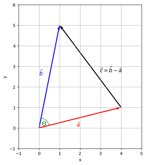
This relationship is shown in Figure 2

^{Figure 2 Three vectors a, b, c. The angle Theta between a and b can be calculated with the help of the dot-product.}

Plot-Code (Python)

import numpy as np
import matplotlib.pyplot as plt
from matplotlib.patches import Arc


a = np.array([4, 1])
b = np.array([1, 5])
c = b - a

a_len = np.linalg.norm(a)
b_len = np.linalg.norm(b)

dot_prod = np.dot(a, b)
cos_theta = dot_prod / (a_len * b_len)
theta_rad = np.arccos(cos_theta)
theta_deg = np.degrees(theta_rad)

angle_a = np.degrees(np.arctan2(a[1], a[0]))

theta1 = angle_a
theta2 = angle_a + theta_deg

fig, ax = plt.subplots(figsize=(6, 6))

ax.quiver(0, 0, a[0], a[1], angles='xy', scale_units='xy', scale=1, color='red')
ax.text(a[0] / 2, a[1] / 2 - 0.5, r'$\vec{a}$', color='red', fontsize=12, ha='right', va='bottom')

ax.quiver(0, 0, b[0], b[1], angles='xy', scale_units='xy', scale=1, color='blue')
ax.text(b[0] / 2 - 0.5, b[1] / 2, r'$\vec{b}$', color='blue', fontsize=12, ha='left', va='bottom')

ax.quiver(a[0], a[1], c[0], c[1], angles='xy', scale_units='xy', scale=1, color='black')
ax.text(a[0] + c[0] / 2 + 1, a[1] + c[1] / 2, r'$\vec{c} = \vec{b} - \vec{a}$', color='black', fontsize=12, ha='center', va='top')

arc = Arc((0, 0), 1.0, 1.0, angle=0, theta1=theta1, theta2=theta2, edgecolor='green')
ax.add_patch(arc)
ax.text(0.11, 0.11, r"$\Theta$", color='green', fontsize=14)

ax.set_xlim(-1, 5)
ax.set_ylim(-1, 6)
ax.set_aspect('equal')
ax.set_xlabel("x")
ax.set_ylabel("y")
ax.grid(True)

plt.show()

First of all, let's substitute the variables with scalar values of our vectors $\vec{a}, \vec{b}$ and $\vec{c}$:

$$|\vec{c}|^2 = |\vec{a}|^2 + |\vec{b}|^2 - 2|\vec{a}||\vec{b}| \cos(\Theta)$$

Note that $\vec{c} = \vec{b} - \vec{a}$, so we can substitute this, too. Additionally, $|c|^2 = \vec{c}^2$:

$$(\vec{b} - \vec{a})^2 = |\vec{a}|^2 + |\vec{b}|^2 - 2|\vec{a}||\vec{b}| \cos(\Theta)$$

We will start with simplifying the terms:

$$\begin{align*} - 2|\vec{a}||\vec{b}| \cos(\Theta) &= (\vec{b} - \vec{a})^2 - |\vec{a}|^2 - |\vec{b}|^2 \\ &= \vec{b}^2 - 2 \vec{a}\vec{b} + \vec{a}^2 - |\vec{a}|^2 - |\vec{b}|^2 \\ &= |\vec{b}|^2 - 2 \vec{a}\vec{b} + |\vec{a}|^2 - |\vec{a}|^2 - |\vec{b}|^2 \\ &= - 2 \cdot (\vec{a} \boldsymbol{\cdot} \vec{b}) \end{align*}$$

Observe that the resulting term on the right side represents the dot product (set in parentheses for clarity).

Finally, solve for $\cos(\Theta)$:

$$\begin{alignat*}{} & -2|\vec{a}||\vec{b}| \cos(\Theta) &&= - 2 \vec{a}\vec{b} \\ \Leftrightarrow \qquad & |\vec{a}||\vec{b}| \cos(\Theta) &&= \vec{a} \boldsymbol{\cdot} \vec{b} \\ \Leftrightarrow \qquad & \cos(\Theta) &&= \frac{\vec{a} \boldsymbol{\cdot} \vec{b}}{|\vec{a}||\vec{b}|} \\ \end{alignat*}{}$$

Clearly, this holds for any vector except for $\vec{a} = \vec{0} \lor \vec{b} = \vec{0}$.

We can now solve for the dot product:

$$\begin{alignat*}{} \vec{a} \boldsymbol{\cdot} \vec{b} = \cos(\Theta) \cdot |\vec{a}||\vec{b}| \end{alignat*}{}$$

The relation between the orthogonality of $\vec{a}$ and $\vec{b}$ and $\Theta = 90 \degree$ becomes more apparent when we consider

$$\begin{alignat*}{} \cos(90\degree) = 0 = \frac{\vec{a} \boldsymbol{\cdot} \vec{b}}{|\vec{a}||\vec{b}|} \end{alignat*}{}$$

Since $|\vec{a}| \neq 0 \land |\vec{b}| \neq 0$ by definition, it follows that $\vec{a} \boldsymbol{\cdot} \vec{b} = 0$. We obtain the equivalence:

$$\vec{a} \boldsymbol{\cdot} \vec{b} = 0 \Leftrightarrow \cos(\Theta) = 0$$

info

The dot product $\vec{a} \boldsymbol{\cdot} \vec{b} = \cos(\Theta) \cdot |\vec{a}||\vec{b}|$ beautifully shows that $\Theta$ is invariant under changes in the magnitude of the related vectors: Using the associativity of the dot product and scalar multiplication, we can derive:

$$\begin{align*} \frac{\vec{a} \boldsymbol{\cdot} \vec{b}}{|\vec{a}| \cdot |\vec{b}|} &= (\vec{a} \boldsymbol{\cdot} \vec{b}) \cdot \frac{1}{|\vec{a}| \cdot |\vec{b}|}\\[1.2em] &= \vec{a} \cdot \frac{1}{|\vec{a}|} \cdot \vec{b} \cdot \frac{1}{|\vec{b}|}\\[1.2em] &= \frac{\vec{a}}{|\vec{a}|} \cdot \frac{\vec{b}}{|\vec{b}|}\\[0.5em] \end{align*}$$

Hence, the cosine of the angle between $\vec{a}$ and $\vec{b}$

$$\begin{align*} \cos(\Theta) = \frac{\vec{a}}{|\vec{a}|} \cdot \frac{\vec{b}}{|\vec{b}|}\\[0.5em] \end{align*}$$

is simply the dot product of the corresponding unit vectors.

Referring back to the introductory example involving the unit circle, observe that $|\vec{a}| = |\vec{b}| = 1$. In this case, the dot product conveniently simplifies:

$$\begin{align*} \vec{a} \boldsymbol{\cdot} \vec{b} = \cos(\Theta) \cdot |\vec{a}||\vec{b}| = \cos(\Theta) \cdot 1 = \cos(\Theta) \end{align*}$$

Using the usual mathematical notation for unit vectors, this can be written as

$$\hat{a} \boldsymbol{\cdot} \hat{b} = \cos(\Theta)$$

Proofs

Proof 1

Let $\vec{a}, \vec{b} \in \mathbb{R}^2$, $\vec{a} \cdot \vec{a} = 1$, $\vec{b} \cdot \vec{b} = 1$, $\vec{a} \boldsymbol{\cdot} \vec{b} = 0$.

Claim: There exists no $\vec{v}$ such that $\vec{v} \neq \vec{a}$, $\vec{v} \cdot \vec{v} = 1$ and $\vec{v} \cdot \vec{b} = 0$

Disproof by counterexample:

Choose

$\vec{a} = \begin{pmatrix} 1 \\ 0 \end{pmatrix}$, $\vec{b} = \begin{pmatrix} 0 \\ 1 \end{pmatrix}$, $\vec{v} = \begin{pmatrix} -1 \\ 0 \end{pmatrix}$.

Clearly, $\vec{v} \neq \vec{a}$ and $\vec{v} \cdot \vec{v} = (-1 \cdot -1) + (0 \cdot 0) = 1$. Moreover,

$\vec{a} \boldsymbol{\cdot} \vec{b} = (1 \cdot 0) + (0 \cdot 1) = 0$ and $\vec{v} \cdot \vec{b} = (-1 \cdot 0) + (0 \cdot 1) = 0$

This contradicts the assumption that no such vector $\vec{v}$ exists with $\vec{a} \neq \vec{v}$ and $\vec{b} \cdot \vec{v} = 0$. $\Box$

Proof 2

Let $\vec{a}, \vec{b} \in \mathbb{R}^2$, $\vec{a} \cdot \vec{a} = 1$, $\vec{b} \cdot \vec{b} = 1$, $\vec{a} \boldsymbol{\cdot} \vec{b} = 0$.

Claim: There exists a $\vec{v}$ such that $\vec{v} \cdot \vec{v} = 1$, $\vec{v} \cdot \vec{a} = 0$ and $\vec{v} \cdot \vec{b} = 0$

Proof by contradiction:

It is clear that $\vec{a}, \vec{b}$ must be perpendicular, or otherwise $\vec{a} \boldsymbol{\cdot} \vec{b} \neq 0$.

Lemma 1:

$\vec{a}$ and $\vec{b}$ are an orthonormal basis of $\mathbb{R}^2$.

Proof of Lemma 1:

For $\vec{a}$, $\vec{b}$ (and $\vec{v}$), the following holds:

$\vec{a} \cdot \vec{a} = (a_x \cdot a_x) + (a _y \cdot a_y) = a^2_x + a^2_y = \sqrt{a^2_x + a^2_y} \cdot \sqrt{a^2_x + a^2_y} = \|a\|^2$

Because of $\vec{a} \cdot \vec{a} = 1$ and $\sqrt{1} = 1$, it follows that $\vec{a}$, $\vec{b}$ must be unit vectors. Since they are perpendicular, they also provide an orthonormal base for $\mathbb{R}^2$. $\Box$

Thus, we can write $\vec{v}$ as a linear combination of $\vec{a}$ and $\vec{b}$:

$\vec{v} = x\vec{a} + y\vec{b}$

We now show that

$\vec{v} \cdot \vec{a} = 0$

$\vec{v} \cdot \vec{b} = 0$

cannot hold:

$\vec{v}$ is perpendicular to both $\vec{a}$ and $\vec{b}$, which are basis vectors of $\mathbb{R}^2$, thus perpendicular to each other. For $\vec{v}$ to be perpendicular to both basis vectors, it follows that $\vec{v}$ itself must be $\vec{0}$, contrary to the assumption that $\vec{v} \cdot \vec{v} = 1$, which implies $\vec{v} \neq \vec{0}$.

info

Additionally, note how $\vec{v}$ is a linear combination of $\vec{a}$ and $\vec{b}$:

$\vec{v} = x\vec{a} + y\vec{b}$

For $\vec{v} \cdot \vec{a} = 0$ and $\vec{v} \cdot \vec{b} = 0$ to hold, $\vec{v}$ must be perpendicular to $\vec{a}$ and to $\vec{b}$.

Since $\vec{a} \ne 0$, but $\vec{v} \cdot \vec{a} = 0$, it follows that $x = 0$, which implies that $\vec{v} = y \vec{b}$. In this case, $\vec{v} \cdot \vec{b} = 0$ must hold, which can only be true if $y = 0$ since $\vec{b} \ne \vec{0}$. This also shows that $\vec{v}$ must be $\vec{0}$.

$\Box$