Rotations as a Special Case of Vector Transformations

Rotations, as a class of linear vector transformations¹, represent rigid body transformations that change the direction of a vector within a given plane.
Efficient and accurate handling of such transformations poses challenges not only for game and animation engines, but also for simulations and real-time systems, where the limitations of floating-point arithmetic and operation throughput can negatively impact the computational outcomes ([📖She97], [📖Kui99]).

This work introduces vector rotation with a focus on the relations between its two- and three-dimensional formulations.

We begin in the two-dimensional plane by deriving classical rotation matrices from linear combinations in orthogonal bases.

We then generalize this approach by introducing Rodrigues' rotation formula, which provides a compact expression for rotation around arbitrary axes in three-dimensional space. We verify that the standard rotation matrices emerge as special cases from this general form.

Finally, we illustrate the application of vector rotation in the context of embedded coordinate systems within large scene graphs, demonstrating how transformations propagate across hierarchical structures in real-time environments such as video games.

Vector Rotation as a Linear Combination

Given an angle $\Theta$ and an orthonormal basis in three-dimensional space, rotating a vector $\vec{v}$ around one of the cardinal axes can be computed with a rotation matrix $\boldsymbol{R}(\Theta)$.

The following matrices define rotations about the $x$, $y$ and $z$ axes, respectively:

$$\boldsymbol{R}_x(\Theta) = \begin{pmatrix} &1 &0 &0 \\ &0 &\cos \Theta &-\sin \Theta\\ &0 &\sin \Theta &\cos \Theta \end{pmatrix}$$ $$\boldsymbol{R}_y(\Theta) = \begin{pmatrix} &\cos \Theta & 0 &\sin \Theta\\ &0 &1 &0\\ &-\sin \Theta & 0 &\cos \Theta \end{pmatrix}$$ $$\boldsymbol{R}_z(\Theta) = \begin{pmatrix} &\cos \Theta &-\sin \Theta &0\\ &\sin \Theta &\cos \Theta &0\\ &0 &0 &1 \end{pmatrix}$$

The matrix $\boldsymbol{R}_z$ directly arises from rotating a vector in the two-dimensional $xy$-plane. This connection will be established in the following.

In an orthonormal basis with the standard basis vectors $\vec{x} = \begin{pmatrix} 1\\0\end{pmatrix}$, $\vec{y} = \begin{pmatrix} 0\\1\end{pmatrix}$, any vector of unit length can be expressed as

$$\vec{v} = \begin{pmatrix} \cos \Theta \\ \sin \Theta \end{pmatrix}$$

This follows directly by $\cos \Theta, \sin \Theta$ when writing $\vec{v}$ as a linear combination of the two linear independent vectors $\vec{x}, \vec{y}$:

$$\vec{v} = a \vec{x} + b \vec{y}$$

Substituting $a, b$ with $\cos \Theta$, $\sin \Theta$, we have:

$$\vec{v} = \cos \Theta \begin{pmatrix} 1 \\ 0 \end{pmatrix} + \sin \Theta \begin{pmatrix} 0 \\ 1 \end{pmatrix} = \begin{pmatrix} \cos \Theta \\ \sin \Theta \end{pmatrix}$$

or, as a matrix multiplication

$$\begin{pmatrix} 1 &0 \\ 0 &1 \end{pmatrix} \begin{pmatrix} \cos \Theta \\\sin \Theta \end{pmatrix} = \vec{v}$$

(Observe how $\vec{x}, \vec{y}$ represent the identity matrix $I_{2}$).

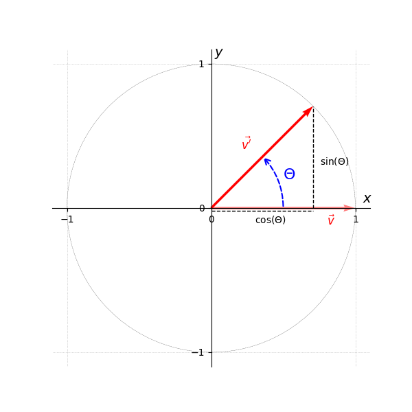
In Figure 1, the angle $\Theta$ represents the amount of rotation of $\vec{v}$ around the origin².

^{Figure 1 The vector v is rotated around the origin by θ degree, resulting in vector v'.}

Plot-Code (Python)

import matplotlib.pyplot as plt
import numpy as np
from matplotlib.patches import Arc, FancyArrowPatch

fig, ax = plt.subplots(figsize=(6, 6))

# Plot setup
ax.set_xlim(-1.1, 1.1)
ax.set_ylim(-1.1, 1.1)
ax.set_xticks([-1, 0, 1])
ax.set_yticks([-1, 0, 1])
ax.set_aspect('equal')
ax.grid(True, linestyle=':', linewidth=0.5)

for spine in ax.spines.values():
    spine.set_visible(False)

ax.spines['bottom'].set_position('zero')
ax.spines['left'].set_position('zero')
ax.spines['bottom'].set_visible(True)
ax.spines['left'].set_visible(True)

ax.xaxis.set_ticks_position('bottom')
ax.yaxis.set_ticks_position('left')

ax.text(1.05, 0.02, r"$x$", fontsize=14, va='bottom')
ax.text(0.02, 1.05, r"$y$", fontsize=14, ha='left')

# Vecors
origin = np.array([0, 0])
theta = np.radians(45)
cos_theta = np.cos(theta)
sin_theta = np.sin(theta)
opposite = np.array([0, np.sin(theta)])
v1 = np.array([np.cos(theta), np.sin(theta)])
v2 = np.array([1, 0])

ax.quiver(*origin, *v1, angles='xy', scale_units='xy', scale=1,  color='r')
ax.quiver(*origin, *v2, angles='xy', scale_units='xy', scale=1, alpha = 0.5, color='r')

offset = 0.01
ax.text(v1[0] - 0.5, v1[1] -0.3, r"$\vec{v'}$", fontsize=12, color='r')
ax.text(v2[0] - 0.2, v2[1]  -0.12, r"$\vec{v}$", fontsize=12, color='r')

# COSINE
ax.plot([0, cos_theta], [-0.02, -0.02], color='black', linestyle='--', linewidth=1)
ax.text(cos_theta / 2 - 0.05, -0.1, r"$\cos(\Theta)$", fontsize=10)

# SINE
start = np.array([cos_theta, 0])
end = start + opposite
ax.plot([start[0], end[0]], [start[1], end[1]], color='black', linewidth=1, linestyle='--')
ax.text(cos_theta + 0.05, sin_theta / 2 - 0.05, r"$\sin(\Theta)$", fontsize=10)


# Unit Circle
circle = plt.Circle((0, 0), 1, color='black', linewidth=0.2, fill=False, transform=ax.transData, linestyle='--')
ax.add_patch(circle)

arrow = FancyArrowPatch(
    posA=(0.5, 0),
    posB=(np.cos(theta)*0.5, np.sin(theta)*0.51),
    connectionstyle="arc3,rad=0.2",
    arrowstyle='->',
    color='blue',
    linestyle='--',
    mutation_scale=15,
    lw=1.5
)
ax.add_patch(arrow)
ax.text(0.5, 0.2, r"$\Theta$", color='blue', fontsize=16)

plt.show()

We claim that

$$\vec{v} = a \vec{x} + b \vec{y}$$

holds for any orthonormal basis, not necessarily the standard basis (which turns out to be just a special case once we have proven the claim).

We require $\sqrt{a^2 + b^2} = 1$ to ensure that $\vec{v}$ has unit length. This condition is immediately satisfied by choosing $a=\cos \Theta, b = \sin \Theta$, as derived in the following proof.

Expressing the linear combination with cosine and sine

Let $\vec{x}, \vec{y} \in \mathbb{R}^2$, $\vec{x} \cdot \vec{y} = 0$, $|\vec{x}| = |\vec{y}| = 1$, $a, b \in \mathbb{R}_{[0, 1]}$, $a^2 + b ^2 = 1$.

Claim: The linear combination $a\vec{x} + b\vec{y}$ can be written as $\cos(\Theta)\vec{x} + \sin(\Theta)\vec{y}$ and yields a normalized vector $\vec{v}$:

$$\hat{v} = \cos(\Theta)\vec{x} + \sin(\Theta)\vec{y}$$

Proof:

We compute the dot products $\vec{v} \cdot \vec{x}$, $\vec{v} \cdot \vec{y}$ to relate the cosines of the angles $\Theta$ (between $\vec{x}$ and $\vec{v}$) and $\varphi$ (between $\vec{y}$ and $\vec{v}$), respectively:

$$\begin{alignat*}{3} \vec{v} \cdot \vec{x} &= \cos(\Theta) |\vec{v}| |\vec{x}| \\ \vec{v} \cdot \vec{y} &= \cos(\varphi) |\vec{v}| |\vec{y}| \end{alignat*}$$

Since $|\vec{x}| = |\vec{y}| = 1$, we find

$$\begin{alignat*}{3} \vec{v} \cdot \vec{x} &= \cos(\Theta) |\vec{v}|\\ \vec{v} \cdot \vec{y} &= \cos(\varphi) |\vec{v}| \end{alignat*}$$

We now solve for $a$ and $b$. Since $\vec{v} = a\vec{x} + b \vec{y}$, we have

$$\begin{split} \vec{v} \cdot \vec{x} &= (a\vec{x} + b \vec{y}) \cdot \vec{x} \\ &= a(|\vec{x}|^2) + b( \vec{x} \cdot \vec{y}) \\ \end{split}$$

Since $\vec{x} \cdot \vec{y} = 0$ and $|\vec{x}| = 1$, we have

$$\begin{split} \vec{v} \cdot \vec{x} = a \\ \end{split}$$

Solving analogously for $b$, we obtain

$$\begin{split} \vec{v} \cdot \vec{y} = b \\ \end{split}$$

We have shown that

$$\begin{alignat*}{3} \vec{v} \cdot \vec{x} &= \cos(\Theta) |\vec{v}| &&= a\\ \vec{v} \cdot \vec{y} &= \cos(\varphi) |\vec{v}| && = b \end{alignat*}$$

and substitute into the linear combination:

$$\begin{alignat*}{3} \vec{v} &= a \vec{x} + b \vec{y} \\ &= \cos(\Theta) |\vec{v}| \vec{x} + \cos(\varphi) |\vec{v}| \vec{y} \end{alignat*}$$

From $\angle(\vec{x}, \vec{y}) = \frac{\pi}{2}$ we can derive

$$\begin{equation}\notag \begin{split} \cos(\varphi) &= \cos(\frac{\pi}{2} - \Theta) \\ &= \cos(\frac{\pi}{2})\cos(\Theta) + \sin(\frac{\pi}{2})\sin(\Theta)\\ &= \sin(\Theta) \end{split} \end{equation}$$

and finally rewrite the linear combination as

$$\vec{v} = \cos(\Theta) |\vec{v}| \vec{x} + \sin(\Theta) |\vec{v}| \vec{y}$$

Dividing by $|\vec{v}|$ yields the normalized vector $\hat{v}$. We therefore receive

$$\frac{\vec{v}}{|\vec{v}|} = \hat{v} = \cos(\Theta) \vec{x} + \sin(\Theta) \vec{y}$$

$\Box$

Verifying the normalization

Under the given assumptions, we verify that $|\hat{v}| = 1$, confirming that $\hat{v}$ is normalized:

$$\begin{equation}\notag \begin{split} |\hat{v}| &= |a \vec{x} + b \vec{y}| \\ &= |a (x_1, x_2)^T + b (y_1, y_2)^T| \\ &= \sqrt{(ax_1 + by_1)^2 + (ax_2 + by_2)^2} \\ &= \sqrt{a^2x_1^2 + a^2x_2^2 + b^2y_1^2 + b^2y_2^2 + 2abx_1y_1 + 2abx_2y_2 } \\ &= \sqrt{a^2(x_1^2 + x_2^2) + b^2(y_1^2 + y_2^2) + 2ab(x_1y_1 + x_2y_2)} \\ &= \sqrt{a^2(\vec{x} \cdot \vec{x} ) + b^2(\vec{y} \cdot \vec{y}) + 2ab(\vec{x} \cdot \vec{y})} \\ &= \sqrt{a^2 + b^2 + 2ab0} \\ &= \sqrt{a^2 + b^2} \end{split} \end{equation}$$

In order for $|\hat{v}| = 1$ to hold, it is required that $a^2 + b^2 = 1$, as given by the assumption.

Substituting $a$ and $b$ by $\cos(\Theta)$ and $\sin(\Theta)$, respectively, we confirm that

$$\cos^2(\Theta) + \sin^2(\Theta) = 1$$

$\Box$

Determining the angle θ between the vectors

Claim: $\Theta$ is the angle between $\hat{v}, \vec{x}$.

This follows trivially since we have already shown that both $\hat{v}$ and $\vec{x}$ are unit vectors. By definition of the dot product, we have:

$$\begin{alignat*}{3} \hat{v} \cdot \vec{x} &= \cos(\Theta) |\hat{v}| |\vec{x}| \\ &= \cos(\Theta) \end{alignat*}$$

which is illustrated in Figure 1.

$\Box$

Generalization to arbitrary lengths

One particular result we get from this - and which will be useful when applying rotations in $\mathbb{R}^3$ around arbitrary axes - is the fact that, for any perpendicular vectors $\vec{x}, \vec{y} \in \mathbb{R}^2$, where $|\vec{x}| = |\vec{y}|$, the linear combination

$$\vec{v} = \cos(\Theta) \vec{x} + \sin(\Theta) \vec{y}$$

yields a vector $\vec{v}$ satisfying

$$|\vec{v}| = |\vec{x}| = |\vec{y}|$$

Following the previous proof, we now treat $\vec{x}, \vec{y}$ as vectors with arbitrary, but equal length, resulting in the (normalized) linear combination

$$\hat{v} = \cos(\Theta) \frac{\vec{x}}{|\vec{x}|} + \sin(\Theta)\frac{\vec{y}}{|\vec{y}|}$$

To cancel out the denominators on the right-hand side, we multiply the equation by $|\vec{x}|$³, yielding

$$\hat{v}|\vec{x}| = \cos(\Theta) \vec{x} + \sin(\Theta) \vec{y}$$

Thus, we obtain a vector with the same magnitude as $\vec{x}$ and $\vec{y}$. $\Box$

Rotation around arbitrary points

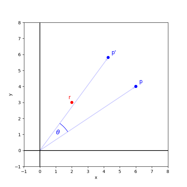
When rotating a point by a given angle, the transformation depends on the chosen center of rotation.

Figure 2 illustrates the point $p = (6, 4)$ rotated by $\Theta = 20 \degree$. Here, $p$ is rotated around the origin $(0, 0)$ of the coordinate plane, resulting in $p'$, which can be obtained via the matrix-vector product

$$\boldsymbol{R}(\Theta) \cdot \vec{p} = \vec{p'}$$

where⁴

$$\boldsymbol{R}(\Theta) = \begin{pmatrix} \cos \Theta & -\sin \Theta \\ \sin \Theta & \cos \Theta \end{pmatrix}$$

^{Figure 2 The point p is rotated around the origin by θ degree, yielding p'.}

Plot-Code (Python)

import numpy as np
import math
import matplotlib.pyplot as plt
from matplotlib.patches import Arc
from matplotlib.ticker import MultipleLocator
from matplotlib.patches import Wedge

# plot layout
fig, ax = plt.subplots(figsize=(6, 6))
ax.set_xlim(-1, 8)
ax.set_ylim(-1, 8)
ax.set_aspect('equal')
ax.set_xlabel("x")
ax.set_ylabel("y")
ax.grid(False)
ax.axhline(0, color='black', linewidth=1.5)
ax.axvline(0, color='black', linewidth=1.5)
ax.xaxis.set_major_locator(MultipleLocator(1))
ax.yaxis.set_major_locator(MultipleLocator(1))

theta = math.radians(20)

p_x = 6
p_y = 4
pc = 'blue'

r_x = 2
r_y = 3
rc = 'red'

# point
p = np.array([p_x, p_y])
p_len = np.linalg.norm(p)

ax.quiver(0, 0, p_x, p_y, angles='xy', scale_units='xy', scale=1, color=pc, width=0.005, linestyle='--',alpha=0.2)

# center of rotation
r = np.array([r_x, r_y])
#ax.quiver(0, 0, r_x, r_y, angles='xy', scale_units='xy', scale=1, color=rc, width=0.005, linestyle='--',alpha=0.2)

# rotated p
pr = np.array([
    p_x * np.cos(theta) - p_y * np.sin(theta),
    p_x * np.sin(theta) + p_y * np.cos(theta)
])
ax.quiver(0, 0, pr[0], pr[1], angles='xy', scale_units='xy', scale=1, color=pc, width=0.005, linestyle='--',alpha=0.2)


circle_p = plt.Circle((p_x, p_y), 0.08, color=pc, fill=True)
ax.add_patch(circle_p)

# p, p'
circle_p = plt.Circle((p_x, p_y), 0.08, color='blue', fill=True)
circle_pr = plt.Circle((pr[0], pr[1]), 0.08, color='blue', fill=True)
ax.add_patch(circle_p)
ax.add_patch(circle_pr)

#r
circle_r = plt.Circle((r_x, r_y), 0.08, color=rc, fill=True)
ax.add_patch(circle_r)

arc_radius = 4.2
arc = Arc((0, 0),
          arc_radius,
          arc_radius,
          angle=0,
          theta1=np.degrees(np.arctan2(p_y, p_x)),
          theta2=20 + np.degrees(np.arctan2(p_y, p_x)),
          edgecolor=pc)
ax.add_patch(arc)

# texts
ax.text(p_x + 0.2, p_y + 0.2, 'p', color=pc, fontsize=12)
ax.text(pr [0] + 0.2, pr[1] + 0.2 , 'p\'', color=pc, fontsize=12)

ax.text(1, 1, r'$\theta$', color=pc, fontsize=14)

ax.text(r_x - 0.2, r_y + 0.2, 'r ', color=rc, fontsize=12)

plt.show()

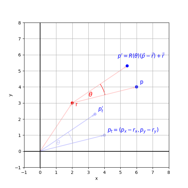
Choosing a different center of rotation

Figure 3 illustrates the rotation around $r$. $\vec{p'}$ is computed such that

• the rotation center $r$ becomes the origin of all points in the coordinate plane
• rotation is applied
• the rotated point is translated back.

Using $\vec{r} = r^T$, we get the expression:

$$\boldsymbol{R}(\Theta) (\vec{p} - \vec{r}) + \vec{r}$$

^{Figure 1 The point p gets translated, then rotated around the origin, then translated back to p'.}

Plot-Code (Python)

import numpy as np
import math
import matplotlib.pyplot as plt
from matplotlib.patches import Arc
from matplotlib.ticker import MultipleLocator
from matplotlib.patches import Wedge

# plot layout
fig, ax = plt.subplots(figsize=(6, 6))
ax.set_xlim(-1, 8)
ax.set_ylim(-1, 8)
ax.set_aspect('equal')
ax.set_xlabel("x")
ax.set_ylabel("y")
ax.grid(False)
ax.axhline(0, color='black', linewidth=1.5)
ax.axvline(0, color='black', linewidth=1.5)
ax.xaxis.set_major_locator(MultipleLocator(1))
ax.yaxis.set_major_locator(MultipleLocator(1))

theta = math.radians(20)

p_x = 6
p_y = 4
pc = 'blue'

r_x = 2
r_y = 3
rc = 'red'

# point
p = np.array([p_x, p_y])
p_len = np.linalg.norm(p)

ax.quiver(0, 0, p_x, p_y, angles='xy', scale_units='xy', scale=1, color=pc, width=0.005, linestyle='--',alpha=0.2)

# center of rotation
r = np.array([r_x, r_y])
#ax.quiver(0, 0, r_x, r_y, angles='xy', scale_units='xy', scale=1, color=rc, width=0.005, linestyle='--',alpha=0.2)

# rotated p
pr = np.array([
    p_x * np.cos(theta) - p_y * np.sin(theta),
    p_x * np.sin(theta) + p_y * np.cos(theta)
])
ax.quiver(0, 0, pr[0], pr[1], angles='xy', scale_units='xy', scale=1, color=pc, width=0.005, linestyle='--',alpha=0.2)


circle_p = plt.Circle((p_x, p_y), 0.08, color=pc, fill=True)
ax.add_patch(circle_p)

# p, p'
circle_p = plt.Circle((p_x, p_y), 0.08, color='blue', fill=True)
circle_pr = plt.Circle((pr[0], pr[1]), 0.08, color='blue', fill=True)
ax.add_patch(circle_p)
ax.add_patch(circle_pr)

#r
circle_r = plt.Circle((r_x, r_y), 0.08, color=rc, fill=True)
ax.add_patch(circle_r)

arc_radius = 4.2
arc = Arc((0, 0),
          arc_radius,
          arc_radius,
          angle=0,
          theta1=np.degrees(np.arctan2(p_y, p_x)),
          theta2=20 + np.degrees(np.arctan2(p_y, p_x)),
          edgecolor=pc)
ax.add_patch(arc)

# texts
ax.text(p_x + 0.2, p_y + 0.2, 'p', color=pc, fontsize=12)
ax.text(pr [0] + 0.2, pr[1] + 0.2 , 'p\'', color=pc, fontsize=12)

ax.text(1, 1, r'$\theta$', color=pc, fontsize=14)

ax.text(r_x - 0.2, r_y + 0.2, 'r ', color=rc, fontsize=12)

plt.show()

Constructing an orthogonal basis for linear combination

As an alternative to explicitly translating a point to the origin, applying rotation and translating it back, we can directly construct an orthogonal basis around $\vec{rp}$ and express the rotated point as a linear combination, as shown in the previous section:

$$\vec{p'} = \cos(\Theta) \vec{rp} + \sin(\Theta) \vec{rp}_{\perp}$$

Here, $\vec{rp}_{\perp}$ is the vector perpendicular to $\vec{rp}$ with the same magnitude, i.e. $|\vec{rp}_{\perp}| = |\vec{rp}|$.

To obtain $\vec{rp}_{\perp}$, we present two practical methods:

1. Using the vector cross product:
   The vector cross product $\vec{w} \times \vec{rp}$ yields a vector $\vec{rp}_{\perp}$ orthogonal to both $\vec{rp}$ and $\vec{w}$.

   $\vec{w}$ is unknown and therefor has to be computed.

   Since the vector cross product is an operation inherently defined in $\mathbb{R}^3$, we need to temporarily extend our vector by a third component: For $\vec{rp}$, we write $(\vec{rp}_x, \vec{rp}_y, 0)$.

   For $\vec{w}$, we choose a unit vector along the $z$-axis, $(0, 0 , 1)^T$, which is perpendicular to our 2-dimensional plane. We then calculate

   $$\vec{rp}_{\perp} = \begin{pmatrix}0 \\ 0 \\ 1\end{pmatrix} \times \begin{pmatrix}\vec{rp}_x \\ \vec{rp}_y \\ 0\end{pmatrix} = \begin{pmatrix} - \vec{rp}_y \\ \vec{rp}_x \\ 0\end{pmatrix}$$

   Dropping the third component in the resulting vector, we end up with $\vec{rp}_{\perp} = (- \vec{rp}_y, \vec{rp}_x)^T$, which is perpendicular to $\vec{rp}$, as verified by their dot product:

   $$(- \vec{rp}_y, \vec{rp}_x)^T \cdot (\vec{rp}_x, \vec{rp}_y)^T = -\vec{rp}_y \vec{rp}_x + \vec{rp}_x \vec{rp}_y = 0$$

   In fact, the resulting vector $\vec{rp}_{\perp}$ is simply $\vec{rp}$ rotated by $90\degree$ counterclockwise, which will be formally verified with the next method.

2. Using the rotation matrix:
   By substituting $\Theta = \frac{\pi}{2}$ ($90\degree$) into the rotation matrix $\boldsymbol{R}(\Theta)$, we get:

   $$\boldsymbol{R}(\frac{\pi}{2}) = \begin{pmatrix}\cos \frac{\pi}{2} & -sin \frac{\pi}{2} \\ \sin \frac{\pi}{2} & \cos \frac{\pi}{2} \end{pmatrix} = \begin{pmatrix}0 & -1 \\ 1 & 0 \end{pmatrix}$$

   Multiplying $\boldsymbol{R}(\frac{\pi}{2})$ with $\vec{rp}$, we obtain the perpendicular vector:

   $$\boldsymbol{R}(\frac{\pi}{2}) \vec{rp} = \begin{pmatrix}0 & -1 \\ 1 & 0 \end{pmatrix} \begin{pmatrix} \vec{rp}_x \\ \vec{rp}_y \end{pmatrix} = \begin{pmatrix} -\vec{rp}_y \\ \vec{rp}_x \end{pmatrix} = \vec{rp}_{\perp}$$

   which also confirms the claim above: $\vec{rp}_{\perp}$ represents $\vec{rp}$ rotated by $90\degree$ ccw.

In both cases, $\vec{rp}_\perp$ can be used for finalizing the linear combination as

$$\vec{p'} = \cos(\Theta) \vec{rp} + \sin(\Theta) \vec{rp}_{\perp}$$

$\Box$

Without delving into the complexity of the involved operations, it should be evident that translating, rotating by $\boldsymbol{R}(\Theta)$, then translating back is more efficient when operating on a large number of vectors, as it avoids computing an orthogonal basis for each case. However, constructing such a basis becomes necessary when rotations around arbitrary axes must be performed, a topic we will address in the next section.

3D Rotation about an Arbitrary Axis

Rodrigues' Rotation Formula

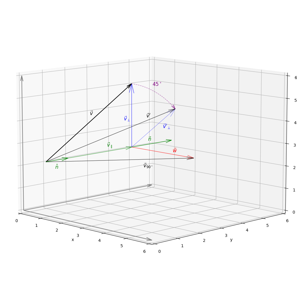
Rotation of vectors about an arbitrary vector $\vec{n} \in \mathbb{R}^3$ in three dimensions involves a combination of vector projection and the use of a locally defined two-dimensional orthogonal basis. The general method for computing such rotations is also known as the Rodrigues formula⁵:

$$\vec{v'} = \vec{v}_{\parallel} + \cos(\Theta) \vec{v}_{\perp} + \sin(\Theta) \vec{w}$$

or, in its commonly used compact form

$$\vec{v}' = \vec{v} \cos(\Theta) + ((\vec{v} \cdot \hat{n}) \cdot \hat{n})(1 - \cos(\Theta)) + (\hat{n} \times \vec{v})\sin(\Theta)$$

We will now proceed to derive the formula, with a special focus on obtaining $\vec{w}$ which represents a coordinate axis in a locally defined orthogonal basis with equal-length axes.

In Figure 4, the vector $\vec{v}$ is rotated about the axis $\vec{n}$. Since we do not care about the magnitude of $\vec{n}$, but rather its direction, we normalize the vector and obtain $\hat{n}$, which will be the center of rotation for $\vec{v}$ in the following derivation.

^{Figure 4 Visualization of Rodrigues' rotation formula applied to vector v, rotated 45° around the axis n. Also shown is the decomposition into the parallel and orthogonal components. A second rotation by 90° demonstrates that the parallel component remains unchanged, while only the perpendicular part (the rejection) undergoes rotation in the locally defined two-dimensional plane.}

Plot-Code (Python)

import matplotlib.pyplot as plt
import numpy as np
import math

def arc(ax, center, v1, v2, theta_start, theta_end, r=1.0, steps=100, **kwargs):
    thetas = np.linspace(theta_start, theta_end, steps)
    arc_points = np.array([
        center + r * (np.cos(t) * v1 + np.sin(t) * v2) for t in thetas
    ])

    if kwargs.get('arrow', True):
        theta = thetas[-1]
        tangent = np.cos(theta)*v2 - np.sin(theta)*v1
        tangent = tangent / np.linalg.norm(tangent)

        arrow_end = arc_points[-1]
        arrow_start = arrow_end - 0.01 * tangent
        ax.quiver(*arrow_start, *tangent, length=0.01,
                  arrow_length_ratio=20, linewidth=1, color=kwargs.get('color', 'black'))

    ax.plot(arc_points[:, 0], arc_points[:, 1], arc_points[:, 2], **kwargs)

def rodrigues(theta, v, n):
    vn = v / np.linalg.norm(v)
    nn = n / np.linalg.norm(n)
    vpar = np.dot(nn, v) * nn
    vperp = v - vpar

    return vpar + (np.cos(theta) * (vperp)) + (np.sin(theta) * np.cross(nn, v))

####################
## CANVAS
####################
fig = plt.figure(figsize=(10, 10))
ax = fig.add_subplot(projection='3d')

ax.set_xlim([0, 6])
ax.set_ylim([0, 6])
ax.set_zlim([0, 6])

ax.set_xlabel('x')
ax.set_ylabel('y')
ax.set_zlabel('z')

ax.quiver(0, 0, 0, 1, 0, 0, color='grey', length=6, arrow_length_ratio=0.04)
ax.quiver(0, 0, 0, 0, 1, 0, color='grey', length=6, arrow_length_ratio=0.04)
ax.quiver(0, 0, 0, 0, 0, 1, color='grey', length=6, arrow_length_ratio=0.04)

ax.view_init(elev=10, azim=-45)


####################
## Parameters
####################
origin = np.array([0, 1, 2])


v = np.array([0, 4, 3])
n = np.array([0, 6, 0])

nn = n / np.linalg.norm(n)

#v
ax.quiver(*origin, *v, color='black',  arrow_length_ratio=0.05)
ax.text(*(v + [0, -2.0, -1.2] + origin), r'$\vec{v}$', color='black', fontsize=12, horizontalalignment='left')

# v parallel
vpar =  np.dot(v, nn) * nn
ax.quiver(*(origin + nn), *(vpar - nn), color='green', linewidth=1, alpha=0.7,  arrow_length_ratio=0.1)
ax.text(*(vpar + [0, -1.2, 0.2] + origin), r'$\vec{v}_{\parallel}$', color='green', fontsize=12, horizontalalignment='left')

#v rotated - demo
vdemo = rodrigues(math.pi / 2, v, n)
ax.quiver(*origin, *vdemo, color='black', linewidth=1, alpha=0.7,  arrow_length_ratio=0.05)
ax.text(*(vdemo + [0, -2.4, -0] + origin), r'$\vec{v}_{90^\circ}$', color='black', fontsize=12, horizontalalignment='left')

#v rotated
vrot = rodrigues(math.pi / 4, v, n)
ax.quiver(*origin, *vrot, color='black', linewidth=1, alpha=0.7,  arrow_length_ratio=0.05)
ax.text(*(vrot + [0, -1.4, -0.2] + origin), r"$\vec{v}'$", color='black', fontsize=12, horizontalalignment='left')

# v perp
vperp = v - vpar
ax.quiver(*(vpar + origin), *vperp, color='blue', linewidth=1, alpha=0.7,  arrow_length_ratio=0.15)
ax.text(*(vpar +[-0.4, 0, 1.2]  + origin), r'$\vec{v}_{\perp}$', color='blue', fontsize=12, horizontalalignment='left')

#w
w = np.cross(nn, v)
ax.quiver(*(vpar + origin), *w, color='red', linewidth=1, alpha=0.7,  arrow_length_ratio=0.1)
ax.text(*(vpar +[2, 0, 0.08] + origin), r'$\vec{w}$', color='red', fontsize=12, horizontalalignment='left')


# v perp 45 degrees
vperp45 = np.cos(math.pi/4) * vperp + np.sin(math.pi/4) * w
ax.quiver(*(vpar + origin), *vperp45, color='blue', linewidth=0.5, alpha=0.7,  arrow_length_ratio=0.15)
ax.text(*(vpar + vperp45 + [0, -0.6, -0.8] + origin), r"$\vec{v}'_{\perp}$", color='blue', fontsize=12, horizontalalignment='left')


#n unit n
ax.quiver(*(origin + vpar), *(n - vpar), color='green', linewidth=1,  arrow_length_ratio=0.15)
ax.text(*(origin + vpar + [0, 0.8, 0.15]), r"$\vec{n}$", color='green', fontsize=12, horizontalalignment='left')

ax.quiver(*origin, *nn, color='green', linewidth=1,  arrow_length_ratio=0.3)
ax.text(*(origin + nn + [0, -0.6, -0.4]), r"$\hat{n}$", color='green', fontsize=12, horizontalalignment='left')


arc(ax, center=origin + vpar, v1=vperp, v2=w,
            theta_start=0, theta_end=np.pi/4, r=1,
            color='purple', alpha=0.5, linewidth=1, linestyle='dashed')
ax.text(*(vrot + [0, -1.1, 1.2] + origin), r'$45^\circ$', color='purple', fontsize=12, horizontalalignment='left')


plt.subplots_adjust(left=0, right=1, top=1, bottom=0)
plt.show()

Clearly, rotating one vector about another vector in 3D must preserve at least one component of the vector that never changes, specifically the one aligned with the axis of rotation. To illustrate this, consider the special case of rotation about one of the standard basis vectors in $\mathbb{R}^3$:

$$\vec{x} = \begin{pmatrix}1 \\ 0 \\ 0\end{pmatrix}, \vec{y} = \begin{pmatrix}0 \\ 1 \\ 0\end{pmatrix}, \vec{z} = \begin{pmatrix}0 \\ 0 \\ 1\end{pmatrix}$$

For example, rotation of a point $(x, y)$ in the Euclidean plane corresponds to rotating the point $(x, y, s)$ in three-dimensional space about the $z$-axis: Here, the $z$-component $s$ always stays unchanged, e.g.

$$\boldsymbol{R}_z(\Theta) \begin{pmatrix}x\\ y\\ s\end{pmatrix} = \begin{pmatrix}x'\\ y'\\ s\end{pmatrix}$$

Analogous reasoning applies to rotation about the $x$-axis and $y$-axis, where the respective components remain constant.

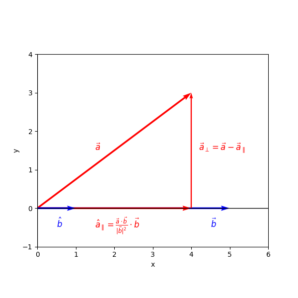
Applying the rules of vector projection in an orthonormal basis - or an orthogonal basis with equal axis lengths, as we will see shortly - helps us isolate the component of a vector that remains unchanged under rotation. Illustrated in Figure 5 is the orthogonal projection of a vector $\vec{a}$ onto another vector $\vec{b}$, which yields the component of $\vec{a}$ parallel to $\vec{b}$.

$$\vec{a}_{\parallel} = \frac{\vec{a} \cdot \vec{b}}{|\vec{b}|^2} \cdot \vec{b}$$

^{Figure 5 Orthogonal projection of a vector a onto a vector b. The projection of a onto b represents the parallel component of vector a into the direction of vector b, the rejection of a from b the component perpendicular to b.}

Plot-Code (Python)

import numpy as np
import math
import matplotlib.pyplot as plt
from matplotlib.patches import Arc
from matplotlib.ticker import MultipleLocator

# plot layout
fig, ax = plt.subplots(figsize=(6, 6))
ax.set_xlim(0, 6)
ax.set_ylim(-1, 4)
ax.set_aspect('equal')
ax.set_xlabel("x")
ax.set_ylabel("y")
ax.grid(False)
ax.axhline(0, color='black', linewidth=1.0)
ax.axvline(0, color='black', linewidth=1.0)
ax.xaxis.set_major_locator(MultipleLocator(1))
ax.yaxis.set_major_locator(MultipleLocator(1))

origin = np.array([0, 0])
a = np.array([4, 3])
b = np.array([5, 0])

bn = b / np.linalg.norm(b)

apar = np.dot(a, bn) * bn
aperp = a - apar

ax.quiver(*origin, *a, angles='xy', scale_units='xy', scale=1, color='red')
ax.quiver(*origin, *b, angles='xy', scale_units='xy', scale=1, color='blue')

ax.quiver(*origin, *apar, angles='xy', scale_units='xy', scale=1, color='red')
ax.quiver(*(origin + apar), *aperp, angles='xy', scale_units='xy', width=0.005, scale=1, color='red')
ax.quiver(*origin, *bn, angles='xy', scale_units='xy', scale=1, color='blue')

ax.text(*(apar + aperp - [-0.2, 1.5]), r'$\vec{a}_{\perp} = \vec{a} - \vec{a}_{\parallel}$', color='red', fontsize=12)
ax.text(*(a - [2.5, 1.5]), r'$\vec{a}$', color='red', fontsize=12)
ax.text(*(bn - [0.5, 0.5]), r'$\hat{b}$', color='blue', fontsize=12)
ax.text(*(apar - apar/2 - [0.5 , 0.5]), r'$\hat{a}_{\parallel} = \frac{\vec{a} \cdot \vec{b}}{|\vec{b}|^2}\cdot\vec{b}$', color='red', fontsize=12)
ax.text(*(b - [0.5, 0.5]), r'$\vec{b}$', color='blue', fontsize=12)

plt.show()

Here, $\vec{a}_{\parallel}$ represents the $x$-component of vector $\vec{a}$ in the direction of $\vec{b}$, while the orthogonal (or "sifted out") $y$-component is given by $\vec{a}_{\perp}$:

$$\vec{a}_{\perp} = \vec{a} - \vec{a}_{\parallel}$$

note

It might at first seem confusing that both the parallel and the perpendicular component change under rotation in two dimensions, whereas we previously stated that the projection parallel to the rotation axis remains constant. This raises the question: Where is the rotation axis located in the Euclidean space? Obviously, there is none, as Foley et al. point out⁶.

This apparent discrepancy resolves once we explicitly construct the rotation axis outside the plane, effectively embedding the plane into a higher dimensional-space.

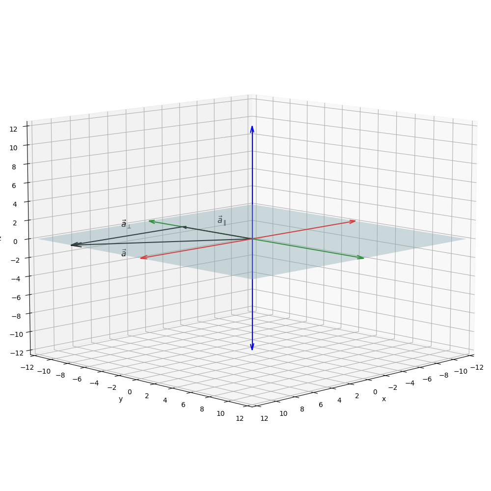
As demonstrated above, a 2D rotation can be represented in 3D by considering vectors lying in an $xy$-plane, perpendicular to the $z$-axis (see Figure 6).

^{Figure 6 Vector a lies in the xy-plane and is rotated around the z-axis. Any projection of a onto the z-axis must be zero since a is perpendicular to z.}

Plot-Code (Python)

import matplotlib.pyplot as plt
import numpy as np
import math


#################
# Canvas
#################
fig = plt.figure(figsize=(10, 10))
ax = fig.add_subplot(projection='3d')

ax.set_xlim([-12, 12])
ax.set_ylim([-12, 12])
ax.set_zlim([-12, 12])

ax.set_xticks(np.arange(-12, 13, 2))
ax.set_yticks(np.arange(-12, 13, 2))
ax.set_zticks(np.arange(-12, 13, 2))

ax.set_xlabel('x')
ax.set_ylabel('y')
ax.set_zlabel('z')

origin = np.array([0, 0, 0])

ax.quiver(*origin, 1, 0, 0, color='red', length=12, arrow_length_ratio=0.06)
ax.quiver(*origin, -1, 0, 0, color='red', length=12, arrow_length_ratio=0.06)
ax.quiver(*origin, 0, 1, 0, color='green', length=12, arrow_length_ratio=0.06)
ax.quiver(*origin, 0, -1, 0, color='green', length=12, arrow_length_ratio=0.06)
ax.quiver(*origin, 0, 0, 1, color='blue', length=12, arrow_length_ratio=0.06)
ax.quiver(*origin, 0, 0, -1, color='blue', length=12, arrow_length_ratio=0.06)

# data
x = np.linspace(-12, 12, 2)
y = np.linspace(-12, 12, 2)
x, y = np.meshgrid(x, y)
z = np.zeros_like(x)
ax.plot_surface(x, y, z, color='lightblue', alpha=0.4)

a = np.array([12, -8, 0])
b = np.array([0, -8, 0])

bn = b / np.linalg.norm(b)

apar = np.dot(a, bn) * bn
aperp = a - apar

ax.quiver(*origin, *a, color='black', length=1, arrow_length_ratio=0.06)
ax.quiver(*origin, *b, color='black', length=1, arrow_length_ratio=0.06)
ax.quiver(*apar, *(aperp), color='black', length=1, arrow_length_ratio=0.06)

ax.text(*origin + [0, -4, 1], r'$\vec{a}_{\parallel}$', color='black', fontsize=12)
ax.text(*origin + [14, 0, 0.5], r'$\vec{a}$', color='black', fontsize=12)
ax.text(*origin + [14, 0, 3.5], r'$\vec{a}_{\perp}$', color='black', fontsize=12)

ax.view_init(elev=10, azim=45)
plt.subplots_adjust(left=0, right=1, top=1, bottom=0)

plt.show()

Here, the orthogonal projection - the parallel component - of any rotated vector onto the rotation axis is always $\vec{0}$ - which corresponds exactly to the situation in two-dimensional rotation. This follows directly from the dot product.

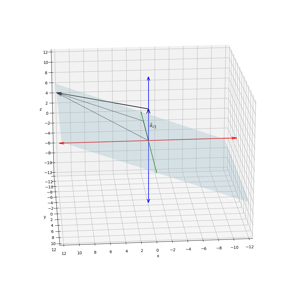
However, once we tilt the plane slightly, such that vectors take the form $(x, y, s)^T$ with $(x, y, s)^T \cdot (0, 0 , 1)^T \neq 0$, the parallel components of these vectors become nonzero and remain fixed under rotation (see Figure 7).

^{Figure 7 The xy-plane is now tilted. Vector a rotates around the z-axis. Unlike before, its projection onto the z-axis is non-zero, yet it remains fixed under rotation.}

Plot-Code (Python)

import matplotlib.pyplot as plt
import numpy as np
import math


#################
# Canvas
#################
fig = plt.figure(figsize=(10, 10))
ax = fig.add_subplot(projection='3d')

ax.set_xlim([-12, 12])
ax.set_ylim([-12, 12])
ax.set_zlim([-12, 12])

ax.set_xticks(np.arange(-12, 13, 2))
ax.set_yticks(np.arange(-12, 13, 2))
ax.set_zticks(np.arange(-12, 13, 2))

ax.set_xlabel('x')
ax.set_ylabel('y')
ax.set_zlabel('z')

origin = np.array([0, 0, 0])

ax.quiver(*origin, 1, 0, 0, color='red', length=12, arrow_length_ratio=0.06)
ax.quiver(*origin, -1, 0, 0, color='red', length=12, arrow_length_ratio=0.06)
ax.quiver(*origin, 0, 1, 0, color='green', length=12, arrow_length_ratio=0.06)
ax.quiver(*origin, 0, -1, 0, color='green', length=12, arrow_length_ratio=0.06)
ax.quiver(*origin, 0, 0, 1, color='blue', length=12, arrow_length_ratio=0.06)
ax.quiver(*origin, 0, 0, -1, color='blue', length=12, arrow_length_ratio=0.06)

# data
tilt = 0.5
x = np.linspace(-12, 12, 10)
y = np.linspace(-12, 12, 10)
x, y = np.meshgrid(x, y)
z = tilt * x
ax.plot_surface(x, y, z, alpha=0.3, color='lightblue')

a = np.array([12, -8, 12 * tilt])
b = np.array([0, -8, 0])
bn = b / np.linalg.norm(b)

apar = np.dot(a, bn) * bn
aperp = a - apar

z = np.array([0, 0, 1])
zn = z / np.linalg.norm(z)
azpar = np.dot(a, zn) * zn
azperp = a - azpar

ax.quiver(*origin, *z, color='black', length=6, arrow_length_ratio=0.06)
ax.quiver(*origin, *azpar, color='black', length=1, arrow_length_ratio=0.15)
ax.quiver(*azpar, *azperp, color='black', length=1, arrow_length_ratio=0.06)

ax.quiver(*origin, *a, color='black', alpha=0.5, length=1, arrow_length_ratio=0.06)
ax.quiver(*origin, *b, color='black', alpha=0.5, length=1, arrow_length_ratio=0.06)
ax.quiver(*apar, *(aperp), color='black', alpha=0.5, length=1, arrow_length_ratio=0.06)

ax.text(*origin + [0, 1, 3], r'$\vec{a}_{z\parallel}$', color='black', fontsize=12)

ax.view_init(elev=20, azim=85)
plt.subplots_adjust(left=0, right=1, top=1, bottom=0)

plt.show()

Informally speaking, the "fixed projection" of a rotated vector in two dimensions is not absent, its just that it's not "visible" within the plane of rotation.

Knowing that the vector-components parallel to the rotation axis stay fixed and only the orthogonal projection changes, we conclude:

• $\vec{v}_{\parallel}$ is the parallel component of $\vec{v}$ onto the normalized rotation axis $\vec{n}$. $\vec{v}_{\parallel}$ can be computed as

  $$\vec{v}_{\parallel} = (\vec{v} \cdot \hat{n}) \cdot \hat{n}$$

  This is the part that never changes during rotation. Thus, the rotated vector $\vec{v}'$ is the vector sum of the parallel projection and the orthogonal projection after rotation.

• $\vec{v}_{\perp}$ is the perpendicular component of $\vec{v}$ and lies in a two-dimensional subspace perpendicular to $\hat{n}$. This component $\vec{v}_{\perp}$, also called the "rejection" of $\vec{v}$ from $\vec{n}$ ([📖Len16, 29]), is obtained by subtracting the parallel component $\vec{v}_{\parallel}$ from $\vec{v}$:

  $$\vec{v}_{\perp} = \vec{v} - \vec{v}_{\parallel}$$

• While the parallel component of $\vec{v}$ stays fixed under rotation, the perpendicular component in respect to the projection changes. It can be expressed by the linear combination

  $$\vec{v}'_{\perp} = \cos(\Theta)\vec{v}_{\perp} + \sin(\Theta)\vec{w}$$

  Here, the locally defined two-dimensional orthogonal basis is given by $\vec{v}_{\perp}$ and the vector $\vec{w}$. For the linear combination to ensure that the resulting vector $\vec{v}'_{\perp}$ has the same length as $\vec{v}_{\perp}$, the vector $\vec{w}$ must have the same magnitude as $\vec{v}_{\perp}$ and correspond to a $90^\circ$ counterclockwise rotation of $\vec{v}_{\perp}$. The existence of such a vector was shown in the previous section. We can obtain the orthogonal basis by computing $\vec{w}$ via

  $$\vec{w} = \hat{n} \times \vec{v}_{\perp}$$

  Since $|\hat{n}| = 1$ and $\angle( \hat{n}, \vec{v}_{\perp}) = \frac{\pi}{2}$, the length of $\vec{w}$ is verified with the vector cross product

  $$|\vec{w}| = |\hat{n} \times \vec{v}_{\perp}|= \sin(\frac{\pi}{2}) \cdot |\hat{n}| \cdot |\vec{v}_{\perp}| = |\vec{v}_{\perp}|$$

Deriving the Rotation Matrices

We now derive $\vec{v}'$ as the result of rotating the vector $\vec{v}$ by an angle $\Theta$ about the rotation axis $\vec{n}$ using the locally defined two-dimensional orthogonal basis, with coordinate axes $\vec{v}_{\perp}$ and $\vec{w}$.

$$\begin{alignat*}{3} \vec{v}' &= \vec{v}_{\parallel} + \cos(\Theta)\vec{v}_{\perp} + \sin(\Theta)\vec{w}\\ &= \vec{v}_{\parallel} + \cos(\Theta)(\vec{v} - \vec{v}_{\parallel}) + \sin(\Theta)(\hat{n} \times \vec{v}_{\perp})\\ &= \vec{v}_{\parallel} + \cos(\Theta)(\vec{v} - (\vec{v} \cdot \hat{n}) \cdot \hat{n}) + \sin(\Theta)(\hat{n} \times (\vec{v} - \vec{v}_{\parallel}))\\ &= \vec{v}_{\parallel} + \cos(\Theta)(\vec{v} - (\vec{v} \cdot \hat{n}) \cdot \hat{n}) + \sin(\Theta)(\hat{n} \times (\vec{v} - (\vec{v} \cdot \hat{n}) \cdot \hat{n}))\\ &= \vec{v}_{\parallel} + \cos(\Theta)(\vec{v} - (\vec{v} \cdot \hat{n}) \cdot \hat{n}) + \sin(\Theta)((\hat{n} \times \vec{v}) - (\hat{n} \times ((\vec{v} \cdot \hat{n}) \cdot \hat{n})))\\ \end{alignat*}$$

which leads to the commonly used compact form of the Rodrigues formula:

$$\vec{v}' = \vec{v} \cos(\Theta) + ((\vec{v} \cdot \hat{n}) \cdot \hat{n})(1 - \cos(\Theta)) + (\hat{n} \times \vec{v})\sin(\Theta)$$

Solving componentwise, we obtain

$$\begin{alignat*}{3} \vec{v}_{\parallel} &= (\vec{v} \cdot \hat{n})\cdot \hat{n} &&= \begin{pmatrix} (\vec{v}_x\hat{n}_x + \vec{v}_y\hat{n}_y + \vec{v}_z\hat{n}_z) \cdot \hat{n}_x \\ (\vec{v}_x\hat{n}_x + \vec{v}_y\hat{n}_y + \vec{v}_z\hat{n}_z) \cdot \hat{n}_y \\ (\vec{v}_x\hat{n}_x + \vec{v}_y\hat{n}_y + \vec{v}_z\hat{n}_z) \cdot \hat{n}_z \end{pmatrix}\\ \\ \ \vec{v}_{\perp} &= \vec{v} - \vec{v}_{\parallel} &&= \begin{pmatrix} \vec{v}_x - (\vec{v}_x\hat{n}_x + \vec{v}_y\hat{n}_y + \vec{v}_z\hat{n}_z) \cdot \hat{n}_x \\ \vec{v}_y - (\vec{v}_x\hat{n}_x + \vec{v}_y\hat{n}_y + \vec{v}_z\hat{n}_z) \cdot \hat{n}_y \\ \vec{v}_z - (\vec{v}_x\hat{n}_x + \vec{v}_y\hat{n}_y + \vec{v}_z\hat{n}_z) \cdot \hat{n}_z \end{pmatrix}\\ \\ \ \vec{w} &= \hat{n} \times \vec{v} &&= \begin{pmatrix} \hat{n}_y\vec{v}_z - \hat{n}_z\vec{v}_y \\ \hat{n}_z\vec{v}_x - \hat{n}_x\vec{v}_z \\ \hat{n}_x\vec{v}_y - \hat{n}_y\vec{v}_x \end{pmatrix} \end{alignat*}$$

Using a specific rotation axis, we verify that $\boldsymbol{R}_z(\Theta)$ follows directly from the Rodrigues formula. We rotate $\vec{v}$ by $\Theta$ around the $z$-axis of the orthonormal standard basis in $\mathbb{R}^3$.

Hence, substituting $\hat{n}$ by $\begin{pmatrix}0 \\ 0\\ 1\end{pmatrix}$ into the formula, we derive $\vec{v}'$:

$$\begin{alignat*}{3} \vec{v}' &= \begin{pmatrix} (\vec{v}_x \cdot 0 + \vec{v}_y \cdot 0 + \vec{v}_z \cdot 1) \cdot 0 \\ (\vec{v}_x \cdot 0 + \vec{v}_y \cdot 0 + \vec{v}_z \cdot 1) \cdot 0 \\ (\vec{v}_x \cdot 0 + \vec{v}_y \cdot 0 + \vec{v}_z \cdot 1) \cdot 1 \end{pmatrix} + \cos(\Theta) \begin{pmatrix} \vec{v}_x - (\vec{v}_x \cdot 0 + \vec{v}_y\cdot 0 + \vec{v}_z\cdot 1) \cdot 0 \\ \vec{v}_y - (\vec{v}_x\cdot 0 + \vec{v}_y\cdot 0 + \vec{v}_z\cdot 1) \cdot 0 \\ \vec{v}_z - (\vec{v}_x\cdot 0 + \vec{v}_y\cdot 0 + \vec{v}_z\cdot 1) \cdot 1 \end{pmatrix} + \sin(\Theta)\begin{pmatrix} 0 \cdot \vec{v}_z - 1 \cdot \vec{v}_y \\ 1\cdot\vec{v}_x - 0\cdot\vec{v}_z \\ 0\cdot\vec{v}_y - 0\cdot\vec{v}_x \end{pmatrix}\\ \\ \ &= \begin{pmatrix} 0 \\ 0 \\ \vec{v}_z \end{pmatrix} + \cos(\Theta) \begin{pmatrix} \vec{v}_x \\ \vec{v}_y \\ 0 \end{pmatrix} + \sin(\Theta)\begin{pmatrix} - \vec{v}_y \\ \vec{v}_x \\ 0 \end{pmatrix}\\ \\ \ &= \begin{pmatrix} \cos(\Theta) \vec{v}_x - \sin(\Theta)\vec{v}_y \\ \cos(\Theta) \vec{v}_y + \sin(\Theta)\vec{v}_x \\ \vec{v}_z \end{pmatrix} \end{alignat*}$$

which corresponds to the matrix-vector product of $\boldsymbol{R}_z(\Theta)$ and $\vec{v}$

$$\begin{alignat*}{3} \vec{v}' &= \begin{pmatrix} \cos(\Theta) \vec{v}_x - \sin(\Theta)\vec{v}_y \\ \cos(\Theta) \vec{v}_y + \sin(\Theta)\vec{v}_x \\ \vec{v}_z \end{pmatrix} \\ \\ \ &= \begin{pmatrix} \cos(\Theta) \vec{v}_x - \sin(\Theta)\vec{v}_y \\ \sin(\Theta)\vec{v}_x + \cos(\Theta) \vec{v}_y \\ \vec{v}_z \end{pmatrix}\\ \\ \ &= \begin{pmatrix} \cos(\Theta) & -\sin(\Theta) & 0 \\ \sin(\Theta) & \cos(\Theta) & 0 \\ 0 & 0 & 1 \end{pmatrix} \cdot \begin{pmatrix} \vec{v}_x \\ \vec{v}_y \\ \vec{v}_z \end{pmatrix}\\ \\ \ &= \boldsymbol{R}_z(\Theta) \vec{v} \end{alignat*}$$

This confirms that the rotation matrix $\boldsymbol{R}_z(\Theta)$ follows directly from Rodrigues' rotation formula.

Similar computations apply to $\boldsymbol{R}_x(\Theta)$ and $\boldsymbol{R}_y(\Theta)$.

Rodrigues’ Rotation Formula in Matrix Form

The following form of Rodrigues’ rotation formula:

$$\vec{v}' = \vec{v} \cos(\Theta) + ((\vec{v} \cdot \hat{n}) \cdot \hat{n})(1 - \cos(\Theta)) + (\hat{n} \times \vec{v})\sin(\Theta)$$

is expanded into matrix form in the following steps.

1. Term $\vec{v} \cos(\Theta)$: Identity component

This term is equivalent to the product of a scaled identity matrix and the vector $\vec{v}$.

$$\begin{pmatrix} \cos \Theta & 0 & 0 \\ 0 & \cos \Theta & 0 \\ 0 & 0& \cos \Theta \end{pmatrix} \vec{v}$$

2. Term $((\vec{v} \cdot \hat{n}) \hat{n})(1 - \cos(\Theta))$: Projection component

We expand $(\vec{v} \cdot \hat{n}) \hat{n}$ explicitly into component form:

$$\begin{alignat*}{3} (\vec{v}_x \hat{n}_x +\vec{v}_y \hat{n}_y + \vec{v}_z \hat{n}_z) \hat{n}_x &= \vec{v}_x \hat{n}^2_x +\vec{v}_y \hat{n}_x\hat{n}_y + \vec{v}_z \hat{n}_x\hat{n}_z\\ (\vec{v}_x \hat{n}_x +\vec{v}_y \hat{n}_y + \vec{v}_z \hat{n}_z) \hat{n}_y &= \vec{v}_x \hat{n}_x\hat{n}_y +\vec{v}_y \hat{n}^2_y + \vec{v}_z \hat{n}_y\hat{n}_z\\ (\vec{v}_x \hat{n}_x +\vec{v}_y \hat{n}_y + \vec{v}_z \hat{n}_z) \hat{n}_z &= \vec{v}_x \hat{n}_x \hat{n}_z +\vec{v}_y \hat{n}_y \hat{n}_z + \vec{v}_z \hat{n}^2_z\\ \end{alignat*}$$

This yields the following matrix representation:

$$\begin{alignat*}{3} \begin{pmatrix} \hat{n}^2_x & \hat{n}_x\hat{n}_y & \hat{n}_x\hat{n}_z\\ \hat{n}_x\hat{n}_y & \hat{n}^2_y & \hat{n}_y\hat{n}_z\\ \hat{n}_x\hat{n}_z & \hat{n}_y\hat{n}_z & \hat{n}^2_z \end{pmatrix} \begin{pmatrix} \vec{v}_x\\ \vec{v}_y\\ \vec{v}_z \end{pmatrix} \end{alignat*}$$

This matrix product is the outer product of $\hat{n}$ with itself and $\vec{v}$:

$$\hat{n} \hat{n}^T \vec{v}$$

with $n_m, v_m$ being the $3 \times 1$ matrix representation (i.e., column vector form) of $\hat{n}$ and $\vec{v}$, respectively:

$$\begin{bmatrix}\begin{pmatrix} \hat{n}_x \\ \hat{n}_y \\ \hat{n}_z \end{pmatrix} \begin{pmatrix} \hat{n}_x & \hat{n}_y & \hat{n}_z \end{pmatrix} \end{bmatrix} \begin{pmatrix} \vec{v}_x \\ \vec{v}_y \\ \vec{v}_z \end{pmatrix}$$

This yields the following matrix expression:

$$\begin{alignat*}{3} \begin{pmatrix} \hat{n}^2_x & \hat{n}_x\hat{n}_y & \hat{n}_x\hat{n}_z\\ \hat{n}_x\hat{n}_y & \hat{n}^2_y & \hat{n}_y\hat{n}_z\\ \hat{n}_x\hat{n}_z & \hat{n}_y\hat{n}_z & \hat{n}^2_z \end{pmatrix}(1 - \cos \Theta)\vec{v} \end{alignat*}$$

3. Term $(\hat{n} \times \vec{v})\sin(\Theta)$: Skew component

This can be expressed using the skew matrix:

$$\begin{pmatrix} 0 & -\hat{n}_z & \hat{n}_y \\ \hat{n}_z & 0 & -\hat{n}_x \\ -\hat{n}_y & \hat{n}_x & 0 \end{pmatrix} (\sin \Theta)\vec{v}$$

4. Final Matrix form of the Rodrigues formula

Combining all three components, the final matrix form of the rotation matrix is:

$$\begin{alignat*}{3} \boldsymbol{R}(\theta, \hat{n}) &= \begin{pmatrix} \cos \Theta & 0 & 0 \\ 0 & \cos \Theta & 0 \\ 0 & 0& \cos \Theta \end{pmatrix} + \begin{pmatrix} \hat{n}^2_x & \hat{n}_x\hat{n}_y & \hat{n}_x\hat{n}_z\\ \hat{n}_x\hat{n}_y & \hat{n}^2_y & \hat{n}_y\hat{n}_z\\ \hat{n}_x\hat{n}_z & \hat{n}_y\hat{n}_z & \hat{n}^2_z \end{pmatrix}(1 - \cos \Theta) + \begin{pmatrix} 0 & -\hat{n}_z & \hat{n}_y \\ \hat{n}_z & 0 & -\hat{n}_x \\ -\hat{n}_y & \hat{n}_x & 0 \end{pmatrix} (\sin \Theta)\\ & \qquad\\ & = \begin{pmatrix} \cos \Theta + \hat{n}^2_x (1 - \cos \Theta) & \hat{n}_x\hat{n}_y (1 - \cos \Theta) -\hat{n}_z \sin \Theta & \hat{n}_x\hat{n}_z (1 - \cos \Theta) + \hat{n}_y \sin \Theta\\ \hat{n}_x\hat{n}_y (1 - \cos \Theta) + \hat{n}_z \sin \Theta & \cos \Theta + \hat{n}^2_y (1 - \cos \Theta) & \hat{n}_y\hat{n}_z (1 - \cos \Theta) -\hat{n}_x \sin \Theta \\ \hat{n}_x\hat{n}_z (1 - \cos \Theta) -\hat{n}_y \sin \Theta & \hat{n}_y\hat{n}_z (1 - \cos \Theta) + \hat{n}_x \sin \Theta & \cos \Theta + \hat{n}^2_z (1 - \cos \Theta) \end{pmatrix} \end{alignat*}$$

By factoring $\vec{v}$ in each term of the expansion, we arrive at a single matrix $\boldsymbol{R}(\Theta, \hat{n})$, which is a composition of a scaled identity, a projection along the rotation axis, and a skew transformation representing the cross product.

Hence, the rotation can be written in one step as

$$\vec{v}' = \boldsymbol{R}(\Theta, \hat{n}) \vec{v}$$

Application: Rodrigues rotation matrix with GLM in C++

When the rotation axis $\vec{n}$ and the rotation angle $\Theta$ are known, a corresponding rotation matrix can be conveniently implemented as a function.

The following C++ function returns a glm::mat3 representing a rotation around an arbitrary axis, using GLM (OpenGL Mathematics)⁷:

mat3 Transform::rotate(const float degrees, const vec3& axis) {

    float theta = radians(degrees);

    vec3 n = normalize(axis);

    float cos_theta = cos(theta);
    float sin_theta = sin(theta);
    float t = 1.0f - cos_theta;

    return mat3(
        cos_theta + n.x * n.x * t,
        n.x * n.y * t + n.z * sin_theta,
        n.x * n.z * t - n.y * sin_theta,

        n.x * n.y * t - n.z * sin_theta,
        cos_theta + n.y * n.y * t,
        n.y*n.z * t + n.x * sin_theta,

        n.x * n.z * t + n.y * sin_theta,
        n.y * n.z * t - n.x * sin_theta,
        cos_theta + n.z * n.z * t
    );
}

Given a vector glm::vec3 v, its rotation around the specified axis by $45^\circ$ can be computed as follows:

vec3 vr = rotate(45.0f, axis) * v;

Application: Scene Graphs and Active Object Transformations

In video games and animations, set pieces typically consist of a large number of objects, each requiring individual transformations. Since some of these objects share parent-child-relationships with others (e.g. aggregates), multiple coordinate systems may be involved. Consequently, transformations must be computed with proper consideration of the corresponding (embedded) coordinate systems.

To keep track of these interdependent and independent objects, game and animation engines use hierarchical data structures that serve different puposes, such as discarding objects outside of the view frustum to reduce the cost of culling operations. Depending on the use case, the applied data structure is ultimately an implementation detail ([📖Jas19, 693]).

Figure 9 shows a scene graph as a simplified representation of an in-game scene from the game Clair Obscur: Expedition 33⁸ (Figure 8). The scene depicts a battle sequence in which the camera moves between fixed positions, based on user interaction and decisions made by the game engine while computing NPC AI.

^{Figure 8 Reaper Cultist NPCs (right) from 'Clair Obscur: Expedition 33' have 3 orbs rotating around its upper torso, serving as buffs.}

In the battle scenes depicted in the screenshot, enemies of the type Reaper Cultist have orbs rotating around their upper torso. The scene graph shown in Figure 9 illustrates a simplified model of these NPCs embedded in the scene, including their orbs, which are represented as individual objects. The handling of multiple (geometric) objects sharing the same type is usually an implementation detail and can also be realized using geometric instances ([📖RTR, 796], [📖PF05, 47]).

^{Figure 9 Simplified scene graph for the depicted battle scene in Clair Obscur.}

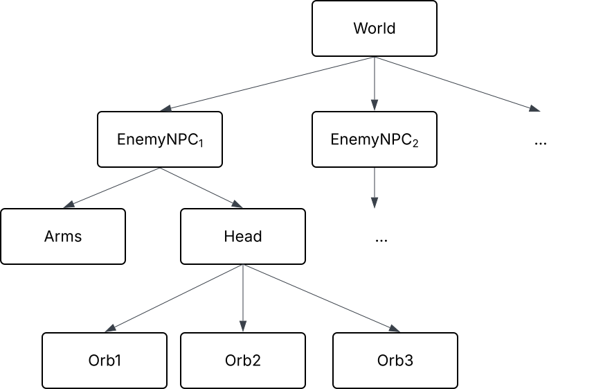
As illustrated by the scene graph, a floating orb is positioned relative to the head of the npc, which in turn is positioned relative to the EnemyNPC$_1$, whose position is defined in world coordinates.

We now abstract the geometric context in Figure 10 to demonstrate how Rodrigues rotation can be applied.

The animation shows a single vector in world coordinates representing EnemyNPC$_1$, along with three spheres arranged around it. The origin of a sphere's local coordinate system is thus defined by the vector's endpoint - i.e. the NPCs head.

Implementing engines must ensure that all vectors are interpreted in the correct context: Since relative positions are provided as points in the coordinate system, it is necessary to derive direction vectors from these positions - typically by computing differences between them and some sort of reference points. For this purpose, any point on the rotation axis can serve as a reference point, because orthogonal projections remain unchanged even if the magnitude of the parallel component varies - as long as the direction remains constant. This is due to the fact that orthogonal and parallel vector components are treated independently in the projection process, as shown in the previous sections.

In these cases, we typically arrive at a composite transformation of the form

$$\vec{v}_{World} = \boldsymbol{T}_{1} \cdot \boldsymbol{T}_{2} \cdot \ldots \cdot \boldsymbol{T}_{n} \cdot \boldsymbol{R}(\Theta, \hat{n}) \cdot \vec{v}_{Object}$$

where the translation matrices $\boldsymbol{T}_i$ successively map each object into the coordinate system of its parent, with transformations applied from right to left ([📖LGK23, 149 ff.]).

Dynamic

^{Figure 10 Visualization of 3 objects rotating around a moving npc. Simplified scene graph for the depicted battle scene in Clair Obscur.}

Plot-Code (Python)

import matplotlib.pyplot as plt
from matplotlib import rcParams
import numpy as np
import math
import random
from matplotlib.animation import FuncAnimation
from IPython.display import HTML
rcParams['animation.embed_limit'] = 50_000_000  # 50 MB

def rodrigues(theta, v, n):
    vn = v / np.linalg.norm(v)
    nn = n / np.linalg.norm(n)
    vpar = np.dot(nn, v) * nn
    vperp = v - vpar

    return vpar + (np.cos(theta) * (vperp)) + (np.sin(theta) * np.cross(nn, v))

fig = plt.figure(figsize=(10, 8))
ax = fig.add_subplot(projection='3d')
plt.subplots_adjust(left=0, right=1, top=1, bottom=0)


npc = np.array([3, 3, 2]) # point coordinates of npc in world
v = np.array([0, 0, 2])   # direction vector of the npc
o1 = np.array([-1, 1, 1])  # orb 1
o2 = np.array([1, 1.5, -1])  # orb2
o3 = np.array([0.5, 3, 0]) # orb 3

theta = 0
end = 360
steps = 2


def init():
    ax.set_xlim([0, 6])
    ax.set_ylim([0, 6])
    ax.set_zlim([0, 6])

    ax.set_xlabel('x')
    ax.set_ylabel('y')
    ax.set_zlabel('z')

    ax.quiver(0, 0, 0, 1, 0, 0, color='grey', length=6, arrow_length_ratio=0.04)
    ax.quiver(0, 0, 0, 0, 1, 0, color='grey', length=6, arrow_length_ratio=0.04)
    ax.quiver(0, 0, 0, 0, 0, 1, color='grey', length=6, arrow_length_ratio=0.04)

    ax.view_init(elev=10, azim=-45)


def update(theta):
    global v
    ax.cla()
    init()
    rad = theta* (math.pi/180)

    sindelta = np.sin(rad*2)
    cosdelta = np.cos(rad*2)

    #npc vector
    origin = np.array([npc[0] + cosdelta/5, npc[1] + sindelta/5, npc[2] + sindelta/1.2]);
    ax.quiver(*origin, *v, color='black', linewidth=4,  arrow_length_ratio=0.05)

    ep1 = rodrigues(rad, [o1[0], o1[1], o1[2] + sindelta/1.2], v)
    ep2 = rodrigues(rad, [o2[0] - cosdelta, o2[1] - sindelta, o2[2] + sindelta/1.25], v)
    ep3 = rodrigues(rad, [o3[0], o3[1], o3[2] + sindelta/1.3], v)

    ax.quiver(*origin + v, *(ep1), color='cyan', linewidth=1,  arrow_length_ratio=0.05)
    ax.quiver(*origin + v, *(ep2), color='cyan', linewidth=1,  arrow_length_ratio=0.05)
    ax.quiver(*origin + v, *(ep3), color='cyan', linewidth=1,  arrow_length_ratio=0.05)


    ax.scatter(*(ep1 + origin + v), color='red', s=100)
    ax.scatter(*(ep2 + origin + v), color='green', s=100)
    ax.scatter(*(ep3 + origin + v), color='blue', s=100)

    theta += steps

ani = FuncAnimation(fig, update, frames=list(range(0, end, steps)), interval=30)
ani.save(
    #path
    writer="pillow",
    fps=30
)

Stationary

^{Figure 11 Visualization of 3 objects rotating around a moving npc. Simplified scene graph for the depicted battle scene in Clair Obscur.}

Plot-Code (Python)

import matplotlib.pyplot as plt
from matplotlib import rcParams
import numpy as np
import math
import random
from matplotlib.animation import FuncAnimation
from IPython.display import HTML

rcParams['animation.embed_limit'] = 50_000_000  # 50 MB

def rodrigues(theta, v, n):
    vn = v / np.linalg.norm(v)
    nn = n / np.linalg.norm(n)
    vpar = np.dot(nn, v) * nn
    vperp = v - vpar

    return vpar + (np.cos(theta) * (vperp)) + (np.sin(theta) * np.cross(nn, v))

fig = plt.figure(figsize=(10, 8))
ax = fig.add_subplot(projection='3d')
plt.subplots_adjust(left=0, right=1, top=1, bottom=0)


npc = np.array([3, 3, 2]) # point coordinates of npc in world
v = np.array([0, 0, 2])   # direction vector of the npc
o1 = np.array([-1, 1, 1])  # orb 1
o2 = np.array([1, 1.5, -1])  # orb2
o3 = np.array([0.5, 3, 0]) # orb 3

theta = 0
end = 360
steps = 2


def init():
    ax.set_xlim([0, 6])
    ax.set_ylim([0, 6])
    ax.set_zlim([0, 6])

    ax.set_xlabel('x')
    ax.set_ylabel('y')
    ax.set_zlabel('z')

    ax.quiver(0, 0, 0, 1, 0, 0, color='grey', length=6, arrow_length_ratio=0.04)
    ax.quiver(0, 0, 0, 0, 1, 0, color='grey', length=6, arrow_length_ratio=0.04)
    ax.quiver(0, 0, 0, 0, 0, 1, color='grey', length=6, arrow_length_ratio=0.04)

    ax.view_init(elev=10, azim=-45)


def update(theta):
    global v
    ax.cla()
    init()
    rad = theta* (math.pi/180)

    sindelta = np.sin(rad*2)
    cosdelta = np.cos(rad*2)

    #npc vector
    origin = npc
    ax.quiver(*origin, *v, color='black', linewidth=4,  arrow_length_ratio=0.05)

    ep1 = rodrigues(rad, [o1[0], o1[1], o1[2] + sindelta/1.2], v)
    ep2 = rodrigues(rad, [o2[0] - cosdelta, o2[1] - sindelta, o2[2] + sindelta/1.25], v)
    ep3 = rodrigues(rad, [o3[0], o3[1], o3[2] + sindelta/1.3], v)

    ax.quiver(*origin + v, *(ep1), color='cyan', linewidth=1,  arrow_length_ratio=0.05)
    ax.quiver(*origin + v, *(ep2), color='cyan', linewidth=1,  arrow_length_ratio=0.05)
    ax.quiver(*origin + v, *(ep3), color='cyan', linewidth=1,  arrow_length_ratio=0.05)


    ax.scatter(*(ep1 + origin + v), color='red', s=100)
    ax.scatter(*(ep2 + origin + v), color='green', s=100)
    ax.scatter(*(ep3 + origin + v), color='blue', s=100)

    theta += steps

ani = FuncAnimation(fig, update, frames=list(range(0, end, steps)), interval=30)
ani.save(
    #path
    writer="pillow",
    fps=30
)

The example above has been deliberately simplified for demonstration purposes, and it should be noted that, in a scene where hundreds of thousands of vertices have to undergo rotation, reducing the computational complexity of operations and improving numerical stability of floating-point computations might be equally important - especially in real-time rendering contexts.
In addition to the Rodrigues formula, Euler angles and quaternions ([📖Ham40]) can be considered for applying rotations in three-dimensional space. Discussions of their respective advantages and limitations are provided by Shoemaker ([📖Sho85]), Hughes et al. ([📖HDMS+14]), and Dunn and Parberry ([📖DP11]).

---

Updates:

• 12.05.2025 Initial publication.
• 17.05.2025 Terminology clarified: More concise and consistent use of orthogonal projection and related vector decomposition concepts.
• 24.05.2025 Added explicit matrix form of Rodrigues' rotation formula.

Footnotes

1. A previous version of this article referred to "affine vector transformations", which is appropriate when considering rotations that also include a translational component. Although such cases are discussed in later sections, the term has been updated to "linear" for conciseness and consistency with the mathematical treatment of pure rotations. ↩

2. See Orthogonality of Unit Vectors ↩

3. Since $|\vec{x}| = |\vec{y}|$, we can also chose $|\vec{y}|$ ↩

4. See Excursus: Constructing a second vector at a specific angle to an existing vector ↩

5. Rodrigues, O. (1840). Des lois géométriques qui régissent les déplacements d'un système solide dans l'espace, et de la variation des coordonnées provenant de ces déplacements considérés indépendamment des causes qui peuvent les produire. Journal de Mathématiques Pures et Appliquées, 5, 380–440. http://eudml.org/doc/234443.
   Friedberg, R. (2022) provides a translation, commentary and additional proofs in his paper Rodrigues, Olinde: "Des lois géométriques qui régissent les déplacements d'un système solide...", translation and commentary. https://arxiv.org/abs/2211.07787. ↩

6. In addition, they provide the proof that rotations in three-dimensional space always have an axis ([📖HDMS+14, 267]). ↩

7. OpenGL Mathematics library for C++: https://github.com/g-truc/glm (retrieved 24.05.2025) ↩

8. Clair Obscur: Expedition 33 is a turn-based RPG developed by the french studio Sandfall Interactive and is published by Kepler Interactive. It was released in April 2025 and to the date of 09.05.2025 the highest ranked PC Game of 2025 on Opencritic ↩

---

References

1. [She97]: Shewchuk, Jonathan R.: Adaptive Precision Floating-Point Arithmetic and Fast Robust Geometric Predicates (1997) [BibTeX]
2. [Kui99]: Kuipers, Jack B.: Quaternions and Rotation Sequences (1999), Princeton University Press [BibTeX]
3. [HDMS+14]: Hughes, John F. and van Dam, Andries and McGuire, Morgan and Sklar, David F. and Foley, James D. and Feiner, Steven K. and Akeley, Kurt: Computer Graphics - Principles and Practice (2014), Addison-Wesley Educational [BibTeX]
4. [Len16]: Lengyel, Eric: Foundations of Game Engine Development, Volume 1: Mathematics (2016), Terathon Software LLC [BibTeX]
5. [Jas19]: Gregory, Jason: Game Engine Architecture (2019), CRC Press [BibTeX]
6. [RTR]: Akenine-Möller, Tomas and Haines, Eric and Hoffman, Naty: Real-Time Rendering (2018), A. K. Peters, Ltd. [BibTeX]
7. [PF05]: Pharr, Matt and Fernando, Randima: GPU Gems 2: Programming Techniques for High-Performance Graphics and General-Purpose Computation (2005), Addison-Wesley Professional [BibTeX]
8. [LGK23]: Lehn, Karsten and Gotzes, Merijam and Klawonn, Frank: Introduction to Computer Graphics: Using OpenGL and Java (2023), Springer, 10.1007/978-3-031-28135-8 [BibTeX]
9. [Ham40]: Hamilton, W. R.: On a New Species of Imaginary Quantities, Connected with the Theory of Quaternions (1840) [BibTeX]
10. [Sho85]: Shoemake, Ken: Animating Rotation with Quaternion Curves (1985), 10.1145/325165.325242 [BibTeX]
11. [DP11]: Dunn, Fletcher and Parberry, Ian: 3D Math Primer for Graphics and Game Development (2011), A K Peters/CRC Press [BibTeX]