The Geometry of the Dot Product

The Dot Product is a fundamental building block for vector operations in video games and simulations. A solid understanding is crucial for applications involving view-related coordinate transformations and even physical modeling within a game world. For many practical use cases, the dot product offers an elegant alternative to constructing explicit visibility cones or relying on computationally expensive raytracing algorithms.

This article provides an introductory exploration of the theory of the dot product and its geometric interpretation.

An example involving field-of-view-calculations illustrates how the dot product can simplify visibility modeling and decision-making in games.

Additional proofs establish key lemmas that support further applications of the dot product and related operations in both 2D and 3D.

Geometric Interpretation

The dot-product takes two vectors and returns the sum of the products of their corresponding components. Given two vectors

$$\vec{a}, \vec {b} \in \mathbb{R}^n, \vec{a} = \begin{pmatrix} a_1 \\ a_2 \\ \vdots \\ a_{n} \end{pmatrix}, \vec{b} = \begin{pmatrix} b_1 \\ b_2 \\ \vdots \\ b_{n} \end{pmatrix}$$

the dot product yields a scalar value.

$$\vec{a} \boldsymbol{\cdot} \vec{b} = \sum_{i=1}^{n} a_ib_i$$

If $\vec{a} \boldsymbol{\cdot} \vec{b} = 0$, the two vectors are perpendicular to each other. We will derive this in the following.

Orthogonality of Unit Vectors

We will first have a look at a special case, namely when $\vec{a}, \vec{b}$ are both unit vectors.

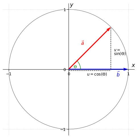
In Figure 1, the radius of the unit circle is represented by the vectors $\vec{a}$ and $\vec{b}$. Thus, for both $\vec{a}$ and $\vec{b}$ the following trivially holds:

$$|\vec{a}| = 1 \\ |\vec{b}| = 1$$

^{Figure 1 Unit Circle with two vectors a and b, which both have a magnitude of 1}

Plot-Code (Python)

import matplotlib.pyplot as plt
import numpy as np
from matplotlib.patches import Arc

fig, ax = plt.subplots(figsize=(6, 6))

# Plot setup
ax.set_xlim(-1.1, 1.1)
ax.set_ylim(-1.1, 1.1)
ax.set_xticks([-1, 0, 1])
ax.set_yticks([-1, 0, 1])
ax.set_aspect('equal')
ax.grid(True, linestyle=':', linewidth=0.5)

for spine in ax.spines.values():
    spine.set_visible(False)

ax.spines['bottom'].set_position('zero')
ax.spines['left'].set_position('zero')
ax.spines['bottom'].set_visible(True)
ax.spines['left'].set_visible(True)

ax.xaxis.set_ticks_position('bottom')
ax.yaxis.set_ticks_position('left')

ax.text(1.05, 0.02, r"$x$", fontsize=14, va='bottom')
ax.text(0.02, 1.05, r"$y$", fontsize=14, ha='left')

# Vecors
origin = np.array([0, 0])
theta = np.radians(45)
cos_theta = np.cos(theta)
sin_theta = np.sin(theta)
opposite = np.array([0, np.sin(theta)])
v1 = np.array([np.cos(theta), np.sin(theta)])
v2 = np.array([1, 0])

ax.quiver(*origin, *v1, angles='xy', scale_units='xy', scale=1, color='r')
ax.quiver(*origin, *v2, angles='xy', scale_units='xy', scale=1, color='b')

offset = 0.01
ax.text(v1[0] - 0.5, v1[1] -0.3, r"$\vec{a}$", fontsize=12, color='r')
ax.text(v2[0] - 0.2, v2[1]  -0.12, r"$\vec{b}$", fontsize=12, color='b')

# COSINE
ax.plot([0, cos_theta], [-0.02, -0.02], color='black', linestyle='--', linewidth=1)
ax.text(cos_theta / 2 - 0.05, -0.1, r"$\cos(\Theta)$", fontsize=10)

# SINE
start = np.array([cos_theta, 0])
end = start + opposite
ax.plot([start[0], end[0]], [start[1], end[1]], color='black', linewidth=1, linestyle='--')
ax.text(cos_theta + 0.05, sin_theta / 2 - 0.05, r"$\sin(\Theta)$", fontsize=10)


# Unit Circle
circle = plt.Circle((0, 0), 1, color='black', linewidth=0.5, fill=False, transform=ax.transData)
ax.add_patch(circle)

# Angle Arc
angle_deg = np.degrees(np.arccos(np.dot(v1, v2)))
arc = Arc(origin, 0.4, 0.4, angle=0, theta1=0, theta2=angle_deg, edgecolor='green')
ax.add_patch(arc)
ax.text(0.08, 0.02, r"$\Theta$", color='green')

plt.show()

Clearly, $\vec{b} = \begin{pmatrix} 1 \\ 0 \end{pmatrix}$.

Additionally $\vec{a} = \begin{pmatrix} cos(\Theta) \\ sin(\Theta) \end{pmatrix}$ can easily be shown since

• the cosine represents the quotient of the adjacent side and the hypotenuse: $cos(\Theta) = \frac{u}{|\vec{a}|}$
• the sine represents the quotient of the opposite side and the hypotenuse: $sin(\Theta) = \frac{v}{|\vec{a}|}$

Solving for $u$ and $v$ respectively gives us

$$cos(\Theta) |\vec{a}| = cos(\Theta) \cdot 1 = cos(\Theta) = u\\ sin(\Theta) |\vec{a}| = sin(\Theta) \cdot 1 = sin(\Theta) = v$$

If $\cos(\Theta) = 0$, it follows directly that $\Theta = 90\degree$.

Orthogonality of Vectors with arbitrary length

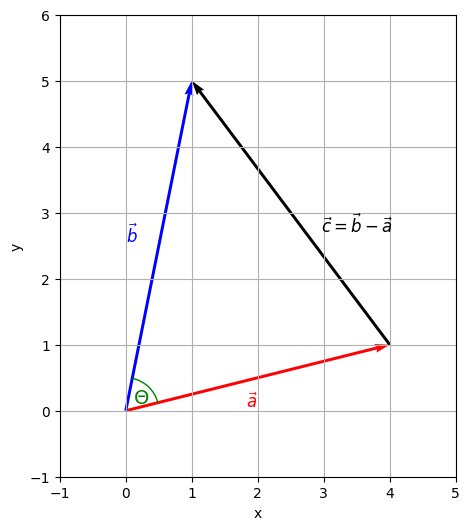
Let's take a look at the common case when $\vec{a}$ and $\vec{b}$ are of arbitrary length and recap the Law of Cosines:

$$c^2 = a^2 + b^2 - 2ab \cos(\Theta)$$

This relationship is shown in Figure 2

^{Figure 2 Three vectors a, b, c. The angle Theta between a and b can be calculated with the help of the dot-product.}

Plot-Code (Python)

import numpy as np
import matplotlib.pyplot as plt
from matplotlib.patches import Arc


a = np.array([4, 1])
b = np.array([1, 5])
c = b - a

a_len = np.linalg.norm(a)
b_len = np.linalg.norm(b)

dot_prod = np.dot(a, b)
cos_theta = dot_prod / (a_len * b_len)
theta_rad = np.arccos(cos_theta)
theta_deg = np.degrees(theta_rad)

angle_a = np.degrees(np.arctan2(a[1], a[0]))

theta1 = angle_a
theta2 = angle_a + theta_deg

fig, ax = plt.subplots(figsize=(6, 6))

ax.quiver(0, 0, a[0], a[1], angles='xy', scale_units='xy', scale=1, color='red')
ax.text(a[0] / 2, a[1] / 2 - 0.5, r'$\vec{a}$', color='red', fontsize=12, ha='right', va='bottom')

ax.quiver(0, 0, b[0], b[1], angles='xy', scale_units='xy', scale=1, color='blue')
ax.text(b[0] / 2 - 0.5, b[1] / 2, r'$\vec{b}$', color='blue', fontsize=12, ha='left', va='bottom')

ax.quiver(a[0], a[1], c[0], c[1], angles='xy', scale_units='xy', scale=1, color='black')
ax.text(a[0] + c[0] / 2 + 1, a[1] + c[1] / 2, r'$\vec{c} = \vec{b} - \vec{a}$', color='black', fontsize=12, ha='center', va='top')

arc = Arc((0, 0), 1.0, 1.0, angle=0, theta1=theta1, theta2=theta2, edgecolor='green')
ax.add_patch(arc)
ax.text(0.11, 0.11, r"$\Theta$", color='green', fontsize=14)

ax.set_xlim(-1, 5)
ax.set_ylim(-1, 6)
ax.set_aspect('equal')
ax.set_xlabel("x")
ax.set_ylabel("y")
ax.grid(True)

plt.show()

First of all, let's substitute the variables with scalar values of our vectors $\vec{a}, \vec{b}$ and $\vec{c}$:

$$|\vec{c}|^2 = |\vec{a}|^2 + |\vec{b}|^2 - 2|\vec{a}||\vec{b}| \cos(\Theta)$$

Note that $\vec{c} = \vec{b} - \vec{a}$, so we can substitute this, too. Additionally, $|c|^2 = \vec{c}^2$:

$$(\vec{b} - \vec{a})^2 = |\vec{a}|^2 + |\vec{b}|^2 - 2|\vec{a}||\vec{b}| \cos(\Theta)$$

We will start with simplifying the terms:

$$\begin{align*} - 2|\vec{a}||\vec{b}| \cos(\Theta) &= (\vec{b} - \vec{a})^2 - |\vec{a}|^2 - |\vec{b}|^2 \\ &= \vec{b}^2 - 2 \vec{a}\vec{b} + \vec{a}^2 - |\vec{a}|^2 - |\vec{b}|^2 \\ &= |\vec{b}|^2 - 2 \vec{a}\vec{b} + |\vec{a}|^2 - |\vec{a}|^2 - |\vec{b}|^2 \\ &= - 2 \cdot (\vec{a} \boldsymbol{\cdot} \vec{b}) \end{align*}$$

Observe that the resulting term on the right side represents the dot product (set in parentheses for clarity).

Finally, solve for $\cos(\Theta)$:

$$\begin{alignat*}{} & -2|\vec{a}||\vec{b}| \cos(\Theta) &&= - 2 \vec{a}\vec{b} \\ \Leftrightarrow \qquad & |\vec{a}||\vec{b}| \cos(\Theta) &&= \vec{a} \boldsymbol{\cdot} \vec{b} \\ \Leftrightarrow \qquad & \cos(\Theta) &&= \frac{\vec{a} \boldsymbol{\cdot} \vec{b}}{|\vec{a}||\vec{b}|} \\ \end{alignat*}{}$$

Clearly, this holds for any vector except for $\vec{a} = \vec{0} \lor \vec{b} = \vec{0}$.

We can now solve for the dot product:

$$\begin{alignat*}{} \vec{a} \boldsymbol{\cdot} \vec{b} = \cos(\Theta) \cdot |\vec{a}||\vec{b}| \end{alignat*}{}$$

The relation between the orthogonality of $\vec{a}$ and $\vec{b}$ and $\Theta = 90 \degree$ becomes more apparent when we consider

$$\begin{alignat*}{} \cos(90\degree) = 0 = \frac{\vec{a} \boldsymbol{\cdot} \vec{b}}{|\vec{a}||\vec{b}|} \end{alignat*}{}$$

Since $|\vec{a}| \neq 0 \land |\vec{b}| \neq 0$ by definition, it follows that $\vec{a} \boldsymbol{\cdot} \vec{b} = 0$. We obtain the equivalence:

$$\vec{a} \boldsymbol{\cdot} \vec{b} = 0 \Leftrightarrow \cos(\Theta) = 0$$

 

The dot product $\vec{a} \boldsymbol{\cdot} \vec{b} = \cos(\Theta) \cdot |\vec{a}||\vec{b}|$ beautifully shows that $\Theta$ is invariant under changes in the magnitude of the related vectors: Using the associativity of the dot product and scalar multiplication, we can derive:

$$\begin{align*} \frac{\vec{a} \boldsymbol{\cdot} \vec{b}}{|\vec{a}| \cdot |\vec{b}|} &= (\vec{a} \boldsymbol{\cdot} \vec{b}) \cdot \frac{1}{|\vec{a}| \cdot |\vec{b}|}\\[1.2em] &= \vec{a} \cdot \frac{1}{|\vec{a}|} \cdot \vec{b} \cdot \frac{1}{|\vec{b}|}\\[1.2em] &= \frac{\vec{a}}{|\vec{a}|} \cdot \frac{\vec{b}}{|\vec{b}|}\\[0.5em] \end{align*}$$

Hence, the cosine of the angle between $\vec{a}$ and $\vec{b}$

$$\begin{align*} \cos(\Theta) = \frac{\vec{a}}{|\vec{a}|} \cdot \frac{\vec{b}}{|\vec{b}|}\\[0.5em] \end{align*}$$

is simply the dot product of the corresponding unit vectors.

Referring back to the introductory example involving the unit circle, observe that $|\vec{a}| = |\vec{b}| = 1$. In this case, the dot product conveniently simplifies:

$$\begin{align*} \vec{a} \boldsymbol{\cdot} \vec{b} = \cos(\Theta) \cdot |\vec{a}||\vec{b}| = \cos(\Theta) \cdot 1 = \cos(\Theta) \end{align*}$$

Using the usual mathematical notation for unit vectors, this can be written as

$$\hat{a} \boldsymbol{\cdot} \hat{b} = \cos(\Theta)$$

Application: Visibility Modeling

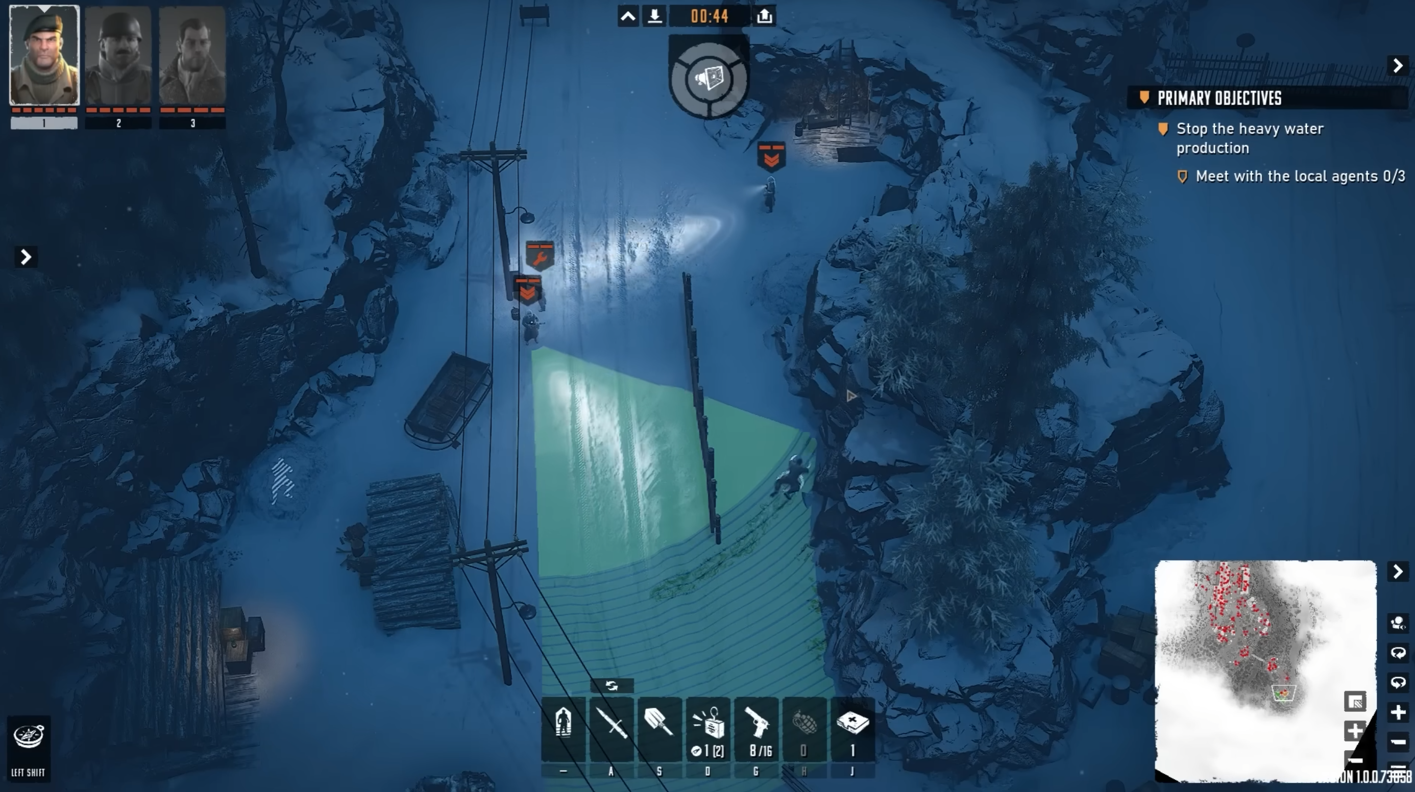
When a game needs to indicate an NPC's Field Of View and its visible range to the player, visibility cones are often used.
A prominent example is Commandos: Behind Enemy Lines¹. Figure 3 shows a screenshot of its recent sequel, Commandos: Origins, where a visibility cone is rendered as a green wedge.

^{Figure 3 An NPC's field of view rendered as a green wedge. The player's character lies directly within the cone. Screenshot grabbed from the IGN review of Commandos: Origins, available at Youtube}

Without considering raytracing for collision detection², the problem of determining whether a given object lies within the visibility cone (and is therefore detected by the game AI) can be simplified to a calculation based solely on the dot product.

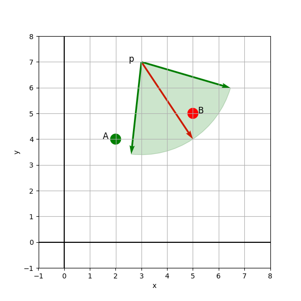
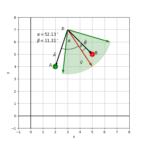
In the following example (see Figure 4), the NPC has the following parameters:

• position $p = (3, 7)$
• view direction $v = (2, -3)
• field of view $f = 80 \degree$
• maximum view distance $|\vec{v}| = \sqrt{13}$

There are two additional characters $A$ $(2, 4)$ and $B$ $(5, 5)$, where $A$ is clearly outside the cone, and $B$ is directly within (similar to the scene shown in Figure 3).

^{Figure 4 To determine if a point lies within the field of view of an NPC, the dot product can be used to calculate the required angles}

Plot-Code (Python)

import numpy as np
import math
import matplotlib.pyplot as plt
from matplotlib.patches import Arc
from matplotlib.ticker import MultipleLocator
from matplotlib.patches import Wedge

# plot layout
fig, ax = plt.subplots(figsize=(6, 6))
ax.set_xlim(-1, 8)
ax.set_ylim(-1, 8)
ax.set_aspect('equal')
ax.set_xlabel("x")
ax.set_ylabel("y")
ax.grid(True)
ax.axhline(0, color='black', linewidth=1.5)
ax.axvline(0, color='black', linewidth=1.5)
ax.xaxis.set_major_locator(MultipleLocator(1))
ax.yaxis.set_major_locator(MultipleLocator(1))

# vectors
fov=80 #fov in degree
v_x = 2
v_y = -3
x = 3
y = 7
v_l = math.sqrt(v_x**2 + v_y**2)

npc = np.array([v_x, v_y])
ax.quiver(x, y, npc[0], npc[1], angles='xy', scale_units='xy', scale=1, color='red')

cos_npc = v_x/v_l
sin_npc = v_y/v_l

theta = np.degrees(np.arccos(cos_npc)) * (-1 if sin_npc < 0 else 1) # *  180 / math.pi
view_left =  theta - (fov/2)
view_right = theta + (fov/2)

v1 = np.array([v_l * np.cos(np.radians(view_left)), v_l * np.sin(np.radians(view_left))])
v2 = np.array([v_l * np.cos(np.radians(view_right)), v_l * np.sin(np.radians(view_right))])

ax.quiver(x, y, v1[0], v1[1], angles='xy', scale_units='xy', scale=1, color='green')
ax.quiver(x, y, v2[0], v2[1], angles='xy', scale_units='xy', scale=1, color='green')


wedge = Wedge(
    center=(3, 7),
    r=v_l,
    theta1=view_left,
    theta2=view_right,
    facecolor='green',
    edgecolor='darkgreen',
    alpha=0.2)

ax.add_patch(wedge)

# A, B
circle_green = plt.Circle((5, 5), 0.2, color='red', fill=True)
circle_red = plt.Circle((2, 4), 0.2, color='green', fill=True)

ax.add_patch(circle_green)
ax.add_patch(circle_red)

# texts
ax.text(2.5, 7 , 'p', color='black', fontsize=12)
ax.text(1.5, 4 , 'A', color='black', fontsize=12)
ax.text(5.2, 5 , 'B', color='black', fontsize=12)

plt.show()

We can now construct two vectors that point from $p$ to $A$ and $B$:

$$\begin{equation}\notag \begin{split} \vec{A} &= A - p = (-1, -3)\\ \vec{B} &= B - p = (2, 2) \end{split} \end{equation}$$

Once we obtain $\hat{A}$, $\hat{B}$, $\hat{v}$, we can utilize the dot product and calculate the cosine of $\alpha$ and $\beta$, i.e. the angles between $\vec{A}$ and $\vec{v}$ and $\vec{B}$ and $\vec{v}$ (see Figure 5).

We solve for $\beta$;

$$\begin{equation}\notag \hat{B} \cdot \hat{v} = \cos(\beta) \approx 0.98 \end{equation}$$

We know that $f/2 = 40\degree$, so $\cos(40\degree) \approx 0.76$.

Since $0.98 > 0.76$³, we conclude that $B$ is within the angular limits defined by the FOV. However, since the length of $\vec{v}$ must also be considered (i.e., the maximum view distance as shown in Figure 4), we have to verify whether $|\vec{B}| \le |\vec{v}|$. In this case, the condition holds, and thus $B$ is confirmed to be within the visibility cone.

^{Figure 5 Using the dot product to calculate angles between the various vectors.}

Plot-Code (Python)

import numpy as np
import math
import matplotlib.pyplot as plt
from matplotlib.patches import Arc
from matplotlib.ticker import MultipleLocator
from matplotlib.patches import Wedge

# plot layout
fig, ax = plt.subplots(figsize=(6, 6))
ax.set_xlim(-1, 8)
ax.set_ylim(-1, 8)
ax.set_aspect('equal')
ax.set_xlabel("x")
ax.set_ylabel("y")
ax.grid(True)
ax.axhline(0, color='black', linewidth=1.5)
ax.axvline(0, color='black', linewidth=1.5)
ax.xaxis.set_major_locator(MultipleLocator(1))
ax.yaxis.set_major_locator(MultipleLocator(1))

# vectors
fov=80 #fov in degree
v_x = 2
v_y = -3
x = 3
y = 7
v_l = math.sqrt(v_x**2 + v_y**2)

npc = np.array([v_x, v_y])
ax.quiver(x, y, npc[0], npc[1], angles='xy', scale_units='xy', scale=1, color='red')

cos_npc = v_x/v_l
sin_npc = v_y/v_l

theta = np.degrees(np.arccos(cos_npc)) * (-1 if sin_npc < 0 else 1) # *  180 / math.pi
view_left =  theta - (fov/2)
view_right = theta + (fov/2)

v1 = np.array([v_l * np.cos(np.radians(view_left)), v_l * np.sin(np.radians(view_left))])
v2 = np.array([v_l * np.cos(np.radians(view_right)), v_l * np.sin(np.radians(view_right))])

ax.quiver(x, y, v1[0], v1[1], angles='xy', scale_units='xy', scale=1, color='green')
ax.quiver(x, y, v2[0], v2[1], angles='xy', scale_units='xy', scale=1, color='green')


wedge = Wedge(
    center=(3, 7),
    r=v_l,
    theta1=view_left,
    theta2=view_right,
    facecolor='green',
    edgecolor='darkgreen',
    alpha=0.2)

ax.add_patch(wedge)

# A, B
circle_green = plt.Circle((5, 5), 0.2, color='red', fill=True)
circle_red = plt.Circle((2, 4), 0.2, color='green', fill=True)

ax.add_patch(circle_green)
ax.add_patch(circle_red)

A = np.array([-1, -3])
ax.quiver(x, y, A[0], A[1], angles='xy', scale_units='xy', scale=1, color='black')
B = np.array([2, -2])
ax.quiver(x, y, B[0], B[1], angles='xy', scale_units='xy', scale=1, color='black')

cos_alpha = np.dot(A, npc) / (np.linalg.norm(A) * np.linalg.norm(npc))
alpha = np.arccos(cos_alpha)
alpha_deg = np.degrees(alpha)
arc_radius_alpha = 3.2
arc_alpha = Arc((3, 7), arc_radius_alpha, arc_radius_alpha,
          angle=np.degrees(np.arctan2(npc[1], npc[0])),
          theta1=-alpha_deg,
          theta2=0,
          edgecolor='black')
ax.add_patch(arc_alpha)

cos_beta = np.dot(B, npc) / (np.linalg.norm(B) * np.linalg.norm(npc))
beta = np.arccos(cos_beta)
beta_deg = np.degrees(beta)
arc_radius_beta = 4.2
arc_beta = Arc((3, 7), arc_radius_beta, arc_radius_beta,
          angle=np.degrees(np.arctan2(npc[1], npc[0])),
          theta1=0,
          theta2=beta_deg,
          edgecolor='black')
ax.add_patch(arc_beta)

# texts
ax.text(2.5, 7 , 'p', color='black', fontsize=12)
ax.text(4, 4.2 , r'$\vec{v}$', color='black', fontsize=12)
ax.text(1.8, 4.8 , r'$\vec{A}$', color='black', fontsize=12)
ax.text(4.3, 5.8 , r'$\vec{B}$', color='black', fontsize=12)
ax.text(1.5, 4 , 'A', color='black', fontsize=12)
ax.text(5.2, 5 , 'B', color='black', fontsize=12)
ax.text(3, 6, rf'$\alpha$', color='black', fontsize=12)
ax.text(4, 5.6, rf'$\beta$', color='black', fontsize=10)
ax.text(0.5, 6.5, rf'$\alpha = {alpha_deg:.2f}^\circ$', color='black', fontsize=12)
ax.text(0.5, 6, rf'$\beta = {beta_deg:.2f}^\circ$', color='black', fontsize=12)

plt.show()

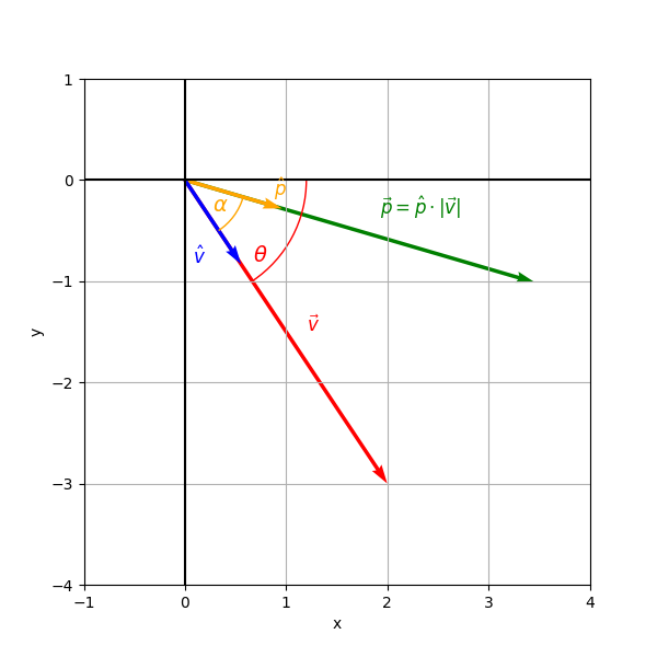
Excursus: Constructing a second vector at a specific angle to an existing vector

 

In the previous example, the view direction of the NPC was given by the vector $\vec{v}$. By using the vector notation, it was also possible to specify the length of the visibility cone, i.e. the maximum range the NPC could see for detecting objects. By applying the dot product to the target's vector $\vec{t}$, we have seen that there is no need for calculating the visibility cone itself - but what if we would like to do so?

One way to obtain vectors at a given angle to a known vector is to take advantage of $\hat{v}$ - the unit vector - in this case, the unit vector of $\vec{v}$:

$$\hat{v} = \frac{\vec{v}}{|\vec{v}|}$$

In Figure 1, we have shown the relationship between sine and cosine as the ratios of the opposite and adjacent sides to the hypotenuse, which represents the radius of the unit circle and is therefore always equal to $1$.

We can use this fact to our advantage by computing a second vector $\vec{p}$ that has the angle $\alpha$ to $\vec{v}$. All we need are the equations

$$\begin{split} \cos(\theta \pm \alpha) &= \cos(\theta)\cos(\alpha) \mp \sin(\theta)\sin(\alpha)\\ \sin(\theta \pm \alpha) &= \sin(\theta)\cos(\alpha) \pm \cos(\theta)\sin(\alpha) \end{split}$$

1. We start with $\cos(\theta + \alpha)$: Since we are using the unit vector $\hat{v}$, we can directly treat $cos(\theta)$ as the $x$-component of $\vec{v}$, and $\sin(\theta)$ as the $y$-component of $\hat{v}$:

   $$\cos(\theta + \alpha) = \hat{v}_x \cdot \cos(\alpha) - \hat{v}_y \cdot \sin(\alpha)$$

   Since the FOV $f$ in the given example is $80 \degree$, we divide $f$ by $2$ to obtain one half of the visibility cone and compute the corresponding direction $\vec{p}$ as follows:

   $$\begin{split} \cos(\theta + 40\degree) &= x\cdot \cos(40\degree) - y \cdot \sin(40\degree)\\ &\approx \hat{v}_x \cdot 0.77 - \hat{v}_y \cdot 0.64\\ &\approx 0.55 \cdot 0.77 - (-0.83 \cdot 0.64)\\ &\approx 0.96 \end{split}$$

2. Compute $\sin(\theta + \alpha)$ analogously:

   $$\begin{split} \sin(\theta + 40\degree) &= y\cdot \cos(40\degree) + x \cdot \sin(40\degree)\\ &\approx \hat{v}_y \cdot 0.77 + \hat{v}_x \cdot 0.64\\ &\approx -0.28 \end{split}$$

The values represent the $\cos(\theta + \alpha) = x$ and $\sin(\theta + \alpha) = y$ components of the desired vector $\vec{p}$, i.e. the ratio between adjacent side and hypotenuse ($x$-direction) and opposite side and hypotenuse ($y$-direction), whereas the hypotenuse is represented by $\hat{v}$. Since we have operated on a unit vector, we obtain a unit vector. Multiplying with any scalar will change the vector's length:

$$\vec{p} = \begin{pmatrix} \cos(\theta + \alpha) \\ \sin(\theta + \alpha) \end{pmatrix} \cdot |\vec{v}|$$

^{Figure 6 Rotating vector v around the origin by 40°. Note that θ is ≈ -56°}

Plot-Code (Python)

import numpy as np
import math
import matplotlib.pyplot as plt
from matplotlib.patches import Arc
from matplotlib.ticker import MultipleLocator

# plot layout
fig, ax = plt.subplots(figsize=(6, 6))
ax.set_xlim(-1, 4)
ax.set_ylim(-4, 1)
ax.set_aspect('equal')
ax.set_xlabel("x")
ax.set_ylabel("y")
ax.grid(True)
ax.axhline(0, color='black', linewidth=1.5)
ax.axvline(0, color='black', linewidth=1.5)
ax.xaxis.set_major_locator(MultipleLocator(1))
ax.yaxis.set_major_locator(MultipleLocator(1))

# vectors
fov = 80  # field of view in degrees
v_x, v_y = 2, -3
v_l = math.sqrt(v_x**2 + v_y**2)

# base vectors
v = np.array([v_x, v_y])
v_u = v / v_l  # unit vector of v

# rotated vector p (by +40°)
angle_offset_deg = 40
theta_v = math.atan2(v_y, v_x)
theta_p = theta_v + math.radians(angle_offset_deg)
p_u = np.array([math.cos(theta_p), math.sin(theta_p)])
p = p_u * v_l

# plot vectors
ax.quiver(0, 0, v[0], v[1], angles='xy', scale_units='xy', scale=1, color='red')
ax.text(v[0]/2 + 0.2, v[1]/2, r'$\vec{v}$', color='red', fontsize=12)

ax.quiver(0, 0, p[0], p[1], angles='xy', scale_units='xy', scale=1, color='green')
ax.text(p[0]/2 + 0.2, p[1]/2 +0.16, r'$\vec{p} = \hat{p} \cdot |\vec{v}|$', color='green', fontsize=12)

# unit vector directions
ax.quiver(0, 0, p_u[0], p_u[1], angles='xy', scale_units='xy', scale=1, color='orange')
ax.text(p_u[0]/2 + 0.4, p_u[1] + 0.12 , r'$\hat{p}$', color='orange', fontsize=12)

ax.quiver(0, 0, v_u[0], v_u[1], angles='xy', scale_units='xy', scale=1, color='blue')
ax.text(v_u[0]/2 - 0.2, v_u[1] , r'$\hat{v}$', color='blue', fontsize=12)

arc_radius = 1.2
arc = Arc((0, 0), arc_radius, arc_radius,
          angle=0,
          theta1=np.degrees(theta_v),
          theta2=np.degrees(theta_p),
          edgecolor='orange')
ax.add_patch(arc)

label_angle = theta_v + (theta_p - theta_v) / 2
label_x = arc_radius * math.cos(label_angle)
label_y = arc_radius * math.sin(label_angle)

arc_radius = 1.2
arc = Arc((0, 0), arc_radius * 2, arc_radius * 2,
          angle=0,
          theta1=-56,
          theta2=0,
          edgecolor='red')
ax.add_patch(arc)
ax.text(label_x - 0.3, label_y - 0.1, r'$\theta$', fontsize=14, color='red')


ax.text(label_x - 0.7, label_y + 0.4, r'$\alpha$', fontsize=14, color='orange')

plt.show()

For the other half of the visibility cone, we simply have to plug $-40\degree$ into the equation.

Rotations of points around a specific axis are performed with the help of rotation matrices. In our 2D-example, the matrix $R$ for rotation around the origin is:

$$R = \begin{pmatrix} \cos(\alpha) & -\sin(\alpha) \\ \sin(\alpha) & \cos(\alpha) \end{pmatrix}$$

By multiplying $R$ with $\vec{v}$⁴, we obtain a new vector rotated $\alpha\degree$ ccw (counterclockwise) around the origin:

$$\begin{pmatrix} \cos(40\degree) & -\sin(40\degree) \\ \sin(40\degree) & \cos(40\degree) \end{pmatrix} \cdot \begin{pmatrix} 2\\-3\end{pmatrix} = \begin{pmatrix} \cos(40\degree) \cdot 2 & +\sin(40\degree) \cdot 3\\ \sin(40\degree) \cdot 2 &- \cos(40\degree) \cdot 3 \end{pmatrix}$$

When applying the cosine/sine addition identity, we first constructed the unit vector $\hat{v}$, rotated it by $40\degree$, and obtained $\hat{p}$. We then scaled $\hat{p}$ by $|\vec{v}|$: This step effectively cancelled out the denominator in the $x$- and $y$-components of $\hat{p}$. It is therefore easy to see that the following holds (in general):

$$R \cdot \vec{v} = R \cdot |\vec{v}| \cdot \hat{v} = |\vec{v}| \cdot R \cdot \hat{v} = |\vec{v}| \cdot \hat{p}$$

Proofs

Uniqueness of Orthogonal Unit Vectors in 2D

Let $\vec{a}, \vec{b} \in \mathbb{R}^2$, $\vec{a} \cdot \vec{a} = 1$, $\vec{b} \cdot \vec{b} = 1$, $\vec{a} \boldsymbol{\cdot} \vec{b} = 0$.

Claim: There exists no $\vec{v}$ such that $\vec{v} \neq \vec{a}$, $\vec{v} \cdot \vec{v} = 1$ and $\vec{v} \cdot \vec{b} = 0$

Disproof by counterexample:

Choose

$\vec{a} = \begin{pmatrix} 1 \\ 0 \end{pmatrix}$, $\vec{b} = \begin{pmatrix} 0 \\ 1 \end{pmatrix}$, $\vec{v} = \begin{pmatrix} -1 \\ 0 \end{pmatrix}$.

Clearly, $\vec{v} \neq \vec{a}$ and $\vec{v} \cdot \vec{v} = (-1 \cdot -1) + (0 \cdot 0) = 1$. Moreover,

$\vec{a} \boldsymbol{\cdot} \vec{b} = (1 \cdot 0) + (0 \cdot 1) = 0$ and $\vec{v} \cdot \vec{b} = (-1 \cdot 0) + (0 \cdot 1) = 0$

This contradicts the assumption that no such vector $\vec{v}$ exists with $\vec{a} \neq \vec{v}$ and $\vec{b} \cdot \vec{v} = 0$. $\Box$

No Third Orthogonal Unit Vector in 2D

Let $\vec{a}, \vec{b} \in \mathbb{R}^2$, $\vec{a} \cdot \vec{a} = 1$, $\vec{b} \cdot \vec{b} = 1$, $\vec{a} \boldsymbol{\cdot} \vec{b} = 0$.

Claim: There exists a $\vec{v}$ such that $\vec{v} \cdot \vec{v} = 1$, $\vec{v} \cdot \vec{a} = 0$ and $\vec{v} \cdot \vec{b} = 0$

Proof by contradiction:

It is clear that $\vec{a}, \vec{b}$ must be perpendicular, or otherwise $\vec{a} \boldsymbol{\cdot} \vec{b} \neq 0$.

Lemma 1:

$\vec{a}$ and $\vec{b}$ are an orthonormal basis of $\mathbb{R}^2$.

Proof of Lemma 1:

For vectors with two components $x, y \in \mathbb{R}$, the following holds in general:

$\vec{a} \cdot \vec{a} = (a_x \cdot a_x) + (a _y \cdot a_y) = a^2_x + a^2_y = \sqrt{a^2_x + a^2_y} \cdot \sqrt{a^2_x + a^2_y} = \|a\|^2$

Because of $\vec{a} \cdot \vec{a} = 1$ and $\sqrt{1} = 1$, it follows that $\vec{a}$, $\vec{b}$ must be unit vectors. Since they are perpendicular, they also provide an orthonormal basis for $\mathbb{R}^2$. $\Box$

Thus, we can write $\vec{v}$ as a linear combination of $\vec{a}$ and $\vec{b}$:

$\vec{v} = x\vec{a} + y\vec{b}$

We now show that

$\vec{v} \cdot \vec{a} = 0$

$\vec{v} \cdot \vec{b} = 0$

cannot hold:

$\vec{v}$ is perpendicular to both $\vec{a}$ and $\vec{b}$, which are basis vectors of $\mathbb{R}^2$, thus perpendicular to each other. For $\vec{v}$ to be perpendicular to both basis vectors, it follows that $\vec{v}$ itself must be $\vec{0}$, contrary to the assumption that $\vec{v} \cdot \vec{v} = 1$, which implies $\vec{v} \neq \vec{0}$.

 

Additionally, note how $\vec{v}$ is a linear combination of $\vec{a}$ and $\vec{b}$:

$\vec{v} = x\vec{a} + y\vec{b}$

For $\vec{v} \cdot \vec{a} = 0$ and $\vec{v} \cdot \vec{b} = 0$ to hold, $\vec{v}$ must be perpendicular to $\vec{a}$ and to $\vec{b}$.

Since $\vec{a} \ne 0$, but $\vec{v} \cdot \vec{a} = 0$, it follows that $x = 0$, which implies that $\vec{v} = y \vec{b}$. In this case, $\vec{v} \cdot \vec{b} = 0$ must hold, which can only be true if $y = 0$ since $\vec{b} \ne \vec{0}$. This also shows that $\vec{v}$ must be $\vec{0}$.

$\Box$

Linear Independence of Orthogonal Vectors in 2D

Let $\vec{a}, \vec{b} \in \mathbb{R}^2$, $\vec{a} \neq \vec{0}, \vec{b} \neq \vec{0}, \vec{a} \cdot \vec{b} = 0$, $\vec{a}$ and $\vec{b}$ are perpendicular to each other.

Claim: $\vec{a}$ and $\vec{b}$ are linearly independent, i.e. $\nexists x, y \neq 0: x\vec{a} + y \vec{b} = \vec{0}$⁵.

Proof by contradiction:

Assume the contrary:

$$\exists x, y \in \mathbb{R}, x, y \neq 0: x\vec{a} + y\vec{b} = \vec{0}$$

Then the following holds:

$$\begin{alignat*}{2} & \qquad \vec{a} \cdot \vec{0} && = 0\\ \Leftrightarrow & \qquad \vec{a} \cdot (x \vec{a} + y \vec{b}) && = 0\\ \Leftrightarrow &\qquad x \vec{a} \cdot \vec{a} + y \vec{a} \cdot \vec{b} && = 0 \\ \Leftrightarrow & \qquad x |\vec{a}|^2 && = - y \vec{a} \cdot \vec{b}\\ \Leftrightarrow & \qquad x |\vec{a}|^2 && = - y \cdot 0\\ \Leftrightarrow & \qquad x |\vec{a}|^2 && = 0 \end{alignat*}$$

$|a| > 0$ since $\vec{a} \neq \vec{0}$. This contradicts the assumption $x \neq 0$. It follows immediately that, if $x = 0$, $y$ must equally be $0$, or otherwise $x\vec{a} + y\vec{b} = \vec{0}$ cannot hold, since $\vec{b} \neq \vec{0}$. $\Box$

info

In general, the following holds: If two vectors $\vec{a}, \vec{b} \in \mathbb{R}^2$ are perpendicular, then they are linearly independent.

Linear combinations of independent vectors span the vector space they belong to - in this case, they create a span for the vector space over $\mathbb{R}^2$ (i.e., the plane $\mathbb{R}^2$).

Note that orthogonality is a sufficient, but not a necessary condition for linear independence: It can be shown that the number of pairs of linearly independent vectors that are not orthogonal, yet create a span over $\mathbb{R}^2$, is infinite (see [📖Axl23, p. 27 ff.]).

---

Footnotes

1. see https://en.wikipedia.org/wiki/Commandos:_Behind_Enemy_Lines ↩

2. Akenine-Möller et al. provide a comprehensive overview of collision detection techniques (including raytracing), available in the freely available appendix of [📖RTR], Real-Time Rendering - Collision Detection ↩

3. $\cos(0\degree) = 1, \cos{90\degree} = 0$. Therefore, the relation $\alpha\degree \le \beta\degree$ is equivalent to $\cos(\alpha\degree) \ge \cos(\beta\degree)$ for $\alpha, \beta \in [0, 90]$ ↩

4. treating the vector as a $2 \times 1$ matrix ↩

5. the equation has only the trivial solution $x=0, y=0$ ↩