Model Matrix: Rotation - World vs. Local Origin

We introduce the mathematical foundation for rotation as linear transformations applied to model matrices in 3D computer graphics and focus on the distinction between rotating an object around an external point and rotating it around its own local origin. We derive the necessary transformations from two conceptually different but mathematically equivalent perspectives: Active transformations, which move the object in a fixed coordinate system, and passive transformations, which redefine the coordinate system around a fixed object. Additionally, we demonstrate the impact of matrix multiplication order, distinguish between world-space and local-space rotations, and conclude with performance considerations and examples from external libraries and game frameworks.

Introduction

The effect of a rotation matrix changes significantly depending on the order of matrix multiplication, as this determines the pivot point for the operation. This article addresses two essential scenarios:

• Rotating an object around an external point¹.
• Rotating an object around its own local origin.

We will derive the mathematical solutions for both cases. The first scenario will be explored from two distinct but equivalent perspectives: as an active transformation that directly manipulates an object's vertices, and as a passive change of coordinates that reorients the coordinate system itself.

By examining the underlying matrix compositions, we will connect this theory to practical examples in common graphics libraries.

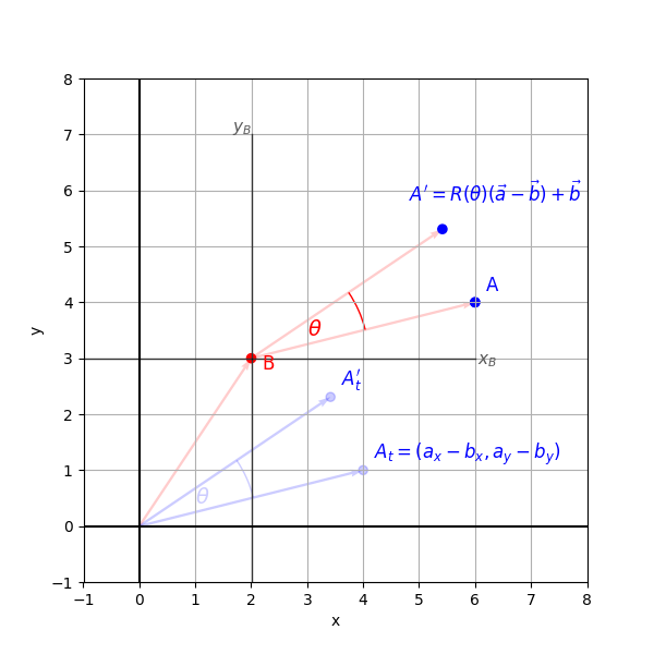
Rotation of A around B

The rotation of an object $A$ around another object $B$ can be seen as the rotation of $A$ around an origin defined by $B$. For this to work, $B$ must be treated as the origin.

In the following, let $A, B \in \mathbb{R}^2$ be points represented by the position vectors $\vec{a}$ and $\vec{b}$, respectively.

Obviously, the position vectors from the world origin (0, 0) to these points are:

$$\begin{alignat*}{3} \vec{b} &= B - 0 \\ \vec{a} &= A - 0 \end{alignat*}$$

We denote the vector pointing from $B$ to $A$ as $\vec{a}_B$. This vector is calculated as:

$$\vec{a}_B = A - B$$

By subtracting $B$'s position from $A$'s, we obtain a direction vector $\vec{a}_B$ which is a direction vector from $B$ - the new origin - to $A$. Applying operations to this new vector is equivalent to performing them in a coordinate system where $B$ is the origin.

For this to work, three steps are necessary:

1. Translation to Origin: The pivot point $B$ is moved to the world origin. This can also be understood as a passive transformation, where the world coordinate system is shifted to align its origin with $B$.
2. Rotation: The object $A$ is then rotated relative to $B$, which is now the (temporary) origin of the world coordinate system.
3. Translate Back: The initial translation is reversed to move the rotated object to its new position within the original coordinate system.

This is illustrated in Figure 1.

^{Figure 1 Point A is first translated so that the pivot point B is at the origin, then rotated around the origin, and finally translated back to its new position, A'. Axes centered at B indicate the coordinate frame of the pivot.}

Plot-Code (Python)

import numpy as np
import math
import matplotlib.pyplot as plt
from matplotlib.patches import Arc
from matplotlib.ticker import MultipleLocator
from matplotlib.patches import Wedge

# plot layout
fig, ax = plt.subplots(figsize=(6, 6))
ax.set_xlim(-1, 8)
ax.set_ylim(-1, 8)
ax.set_aspect('equal')
ax.set_xlabel("x")
ax.set_ylabel("y")
ax.grid(True)
ax.axhline(0, color='black', linewidth=1.5)
ax.axvline(0, color='black', linewidth=1.5)
ax.xaxis.set_major_locator(MultipleLocator(1))
ax.yaxis.set_major_locator(MultipleLocator(1))

theta = math.radians(20)

p_x = 6
p_y = 4
pc = 'blue'

r_x = 2
r_y = 3
rc = 'red'

# point
p = np.array([p_x, p_y])
p_len = np.linalg.norm(p)


# center of rotation
r = np.array([r_x, r_y])
ax.quiver(0, 0, r_x, r_y, angles='xy', scale_units='xy', scale=1, color=rc, width=0.005, linestyle='--',alpha=0.2)

# rotated p
pr = np.array([
    ((p_x - r[0]) * np.cos(theta) - (p_y - r[1]) * np.sin(theta)) + r[0],
    ((p_x - r[0]) * np.sin(theta) + (p_y - r[1]) * np.cos(theta)) + r[1]
])


# vectors from r to p, p'
ax.quiver(r_x, r_y, pr[0] - r_x, pr[1] - r_y, angles='xy', scale_units='xy', scale=1, color=rc, width=0.005, linestyle='--',alpha=0.2)
ax.quiver(r_x, r_y, p[0] - r_x, p[1] - r_y, angles='xy', scale_units='xy', scale=1, color=rc, width=0.005, linestyle='--',alpha=0.2)

# p - r
ax.quiver(0, 0, p_x - r_x, p_y - r_y, angles='xy', scale_units='xy', scale=1, color=pc, width=0.005, linestyle='--',alpha=0.2)
ax.quiver(0, 0, pr[0] - r_x, pr[1] - r_y, angles='xy', scale_units='xy', scale=1, color=pc, width=0.005, linestyle='--',alpha=0.2)

circle_p = plt.Circle((p_x, p_y), 0.08, color=pc, fill=True)
ax.add_patch(circle_p)

# p, p'
circle_p = plt.Circle((p_x, p_y), 0.08, color='blue', fill=True)
circle_pr = plt.Circle((pr[0], pr[1]), 0.08, color='blue', fill=True)
ax.add_patch(circle_p)
ax.add_patch(circle_pr)

circle_pt = plt.Circle((p_x - r_x, p_y - r_y), 0.08, color='blue', fill=True, alpha=0.2)
circle_prt = plt.Circle((pr[0] - r_x, pr[1] - r_y), 0.08, color='blue', fill=True, alpha=0.2)
ax.add_patch(circle_pt)
ax.add_patch(circle_prt)

#r
circle_r = plt.Circle((r_x, r_y), 0.08, color=rc, fill=True)
ax.add_patch(circle_r)

arc_radius = 4.2
arc = Arc((r[0], r[1]),
          arc_radius,
          arc_radius,
          angle=0,
          theta1=np.degrees(np.arctan2(p_y - r[1], p_x - r[0])),
          theta2=20 + np.degrees(np.arctan2(p_y - r[1], p_x - r[0])),
          edgecolor=rc)
ax.add_patch(arc)

arc_radius = 4.2
arc = Arc((0, 0),
          arc_radius,
          arc_radius,
          angle=0,
          theta1=np.degrees(np.arctan2(p_y - r[1], p_x - r[0])),
          theta2=20 + np.degrees(np.arctan2(p_y - r[1], p_x - r[0])),
          alpha=0.2,
          edgecolor=pc)
ax.add_patch(arc)

# texts
ax.text(p_x + 0.2, p_y + 0.2, 'A', color=pc, fontsize=12)
ax.text(pr [0] - 0.6, pr[1] + 0.5 , r"$A' = R(\theta)(\vec{a} - \vec{b}) + \vec{b}$", color=pc, fontsize=12)

ax.text(p_x - r_x + 0.2, p_y - r_y + 0.2, r'$A_t = (a_x - b_x, a_y - b_y)$', color=pc, fontsize=12)
ax.text(pr[0] - r_x + 0.2, pr[1] - r_y + 0.2 , r"$A_t'$", color=pc, fontsize=12)
ax.text(0 + 1, 0 + 0.4, r'$\theta$', color=pc, fontsize=14, alpha=0.2)

ax.text(r_x + 0.2, r_y - 0.2, 'B ', color=rc, fontsize=12)
ax.text(r_x + 1, r_y + 0.4, r'$\theta$', color=rc, fontsize=14)

# axes through B
L = 4
ax.plot([r_x - L, r_x + L], [r_y, r_y], linestyle='-', linewidth=1.0, color='black', alpha=0.7)
ax.plot([r_x, r_x], [r_y - L, r_y + L], linestyle='-', linewidth=1.0, color='black', alpha=0.7)
ax.text(r_x + L + 0.05, r_y - 0.1, r'$x_B$', color='0.35', fontsize=11)
ax.text(r_x - 0.35, r_y + L + 0.05, r'$y_B$', color='0.35', fontsize=11)

plt.show()

Active Transformation

Let $\vec{a}$ be the position vector of the point $A$ we want to rotate, and let $\vec{b}$ be the position vector of the pivot point $B$.

To rotate $A$ around $B$, we first perform an affine transformation that translates $\vec{a}$ into a new coordinate system where B is the origin. This is achieved by subtracting $\vec{b}$ from $\vec{a}$:

$$\vec{a}_B = \vec{a} - \vec{b}$$

The resulting vector, $\vec{a}_{B}$, now points from $B$ to $A$. By performing this transformation, we ensure that subsequent operations, such as applying a rotation matrix $\boldsymbol{R}(\theta)$, will rotate $A$ relative to $B$ - as if $B$ were the origin.

The calculation sequence, understanding the affine transformations as matrices, is as follows:

$$\boldsymbol{T}_{\vec{b}}\ \boldsymbol{R}(\theta)\ \boldsymbol{T}_{-\vec{b}}\ \vec{a}$$

As usual, we interpret this from right to left:

$$\text{translate the rotated result back} \leftarrow \text{rotate the result} \leftarrow \text{Translate }\vec{a}\text{ to the origin}$$

A model matrix, $\boldsymbol{M}$, typically consists of a composition of scaling, rotation, and translation operations. We can express this as a single $4 \times 4$ affine transformation matrix:

$$\boldsymbol{M} = \begin{bmatrix} \boldsymbol{L} & \vec{t} \\ 0 & 1 \end{bmatrix}$$

Here, $\boldsymbol{L}$ is a 3x3 matrix representing the combined linear transformations (scaling and rotation), and $\vec{t}$ is the translation vector.

To transform the object represented by this model matrix so that its pivot point $B$ is at the origin, we pre-multiply its model matrix by a translation matrix $\boldsymbol{T}_{-\vec{b}}$:

$$\boldsymbol{T}_{-\vec{b}} = \begin{bmatrix}\boldsymbol{I}_3 & -\vec{b}\\ 0 & 1\end{bmatrix}$$

By applying the rotation and corresponding back-translation, we get the final composite matrix, M

$$\boldsymbol{M'} = \begin{bmatrix}\boldsymbol{I}_3 & \vec{b}\\ 0 & 1\end{bmatrix} \begin{bmatrix}\boldsymbol{R}_3 & 0\\ 0 & 1\end{bmatrix} \begin{bmatrix}\boldsymbol{I}_3 & -\vec{b}\\ 0 & 1\end{bmatrix} \begin{bmatrix}\boldsymbol{L} & \vec{t} \\0 & 1\end{bmatrix}$$

When a local-space vector $\vec{a}$ is multiplied by this matrix, the transformations are applied from right to left:

$$\vec{a'} = \boldsymbol{M'} \vec{a} = \begin{bmatrix}\boldsymbol{I}_3 & \vec{b}\\ 0 & 1\end{bmatrix} \begin{bmatrix}\boldsymbol{R}_3 & 0\\ 0 & 1\end{bmatrix} \begin{bmatrix}\boldsymbol{I}_3 & -\vec{b}\\ 0 & 1\end{bmatrix} \begin{bmatrix}\boldsymbol{L} & \vec{t} \\0 & 1\end{bmatrix} \ \vec{a}$$

This unfolds in the following sequence:

1. Model to World: First, the local vector $\vec{a}$ is multiplied by the model matrix $\boldsymbol{M}$ This transforms it into world space, resulting in the vector $\vec{a}_W$
2. Translate to Origin: The world-space vector $\vec{a}_W$ is then multiplied by $\begin{bmatrix}\boldsymbol{I}_3 & -\vec{b}\\ 0 & 1\end{bmatrix}$. This actively moves the vector by $-\vec{b}$. The result is the vector's position relative to the pivot point B, $\vec{a}_B$.
3. Rotate: This translated vector is then multiplied by the rotation matrix $\boldsymbol{R}(\theta)$ yields $\vec{a}_R$, rotating it around the world origin (for $\vec{a}_B$, this is now $B$).
4. Translate Back: Finally, the rotated vector is multiplied by $\begin{bmatrix}\boldsymbol{I}_3 & \vec{b}\\ 0 & 1\end{bmatrix}$. This moves the vector back by $\vec{b}$, placing it in its final rotated position in the world.

Since matrix multiplication is associative, we can pre-multiply all the transformation matrices together to create a single, final matrix $\boldsymbol{M'}$. Applying this single matrix $\boldsymbol{M'}$ to the local vector achieves the same result in one operation.

Performance Considerations

When transforming a large number $n$ of vertices, pre-multiplying the transformation matrices into a single matrix is more efficient than applying each matrix to every vector step-by-step. The proof lies in comparing the total number of arithmetic operations.

Let's assume our transformation consists of the four given $4 \times 4$ matrices, and we have a number of $n$ homogenous $4 \times 1$ vertices $\vec{v_i}$. Then, the following holds in our case:

• A dot product of two vectors $\vec{v}_i$, $\vec{v}_j$ requires $4$ multiplications and $3$ additions: $7$ total operations.
• A single matrix-vector multiplication requires $4$ dot products, totaling $16$ multiplications and $12$ additions: $28$ total operations.
• A matrix-matrix multiplication requires $16$ dot products, totaling $64$ multiplications and $48$ additions: $112$ total operations.

Comparing a step-by-step transformation vs. pre-multiplying the matrices yields the following:

Step-by-Step Transformation

For each vertex, we perform four matrix-vector multiplications. This results in a cost per vertex of $4(16+12) = 64+48 = 112$ total operations. Hence, for $n$ vertices, this method requires $112n$ operations.

Pre-Multiplying the Matrix

This involves a one-time setup cost due to calculating $\boldsymbol{M}'$. To obtain $\boldsymbol{M}'$ we need to perform $3 ( 4(16+12)) = 3(64+48) = 336$ total operations. Each vertex has a cost of $16+12 = 28$ operations, hence, for $n$ vertices, this method requires $336 + (28n)$ operations.

Solving the inequality for $n$ gives us

$$336 + (28n) < 112n \Leftrightarrow 4 < n$$

Therefore, pre-multiplying the matrices is more computationally efficient than the step-by-step transformation for more than $4$ vertices² $\Box$

Passive Transformation

Conceptually, the transformation can also be expressed using change-of-coordinates matrices³. In a passive transformation, the vector $\vec{a}$ remains fixed, and its coordinates are expressed in different coordinate systems. To incorporate translations, we represent the vector in homogeneous coordinates, $(a_x, a_y, a_z, 1)^T$, and extend the $3 \times 3$ change-of-basis matrices to $4 \times 4$ affine matrices. We will assume all coordinate systems we consider have orthonormal bases.

First, we create a change-of-basis matrix to express the local vector $[\vec{a}]_A$ in world coordinates:

$$[\vec{a}]_W =\underset{W \leftarrow A}{\boldsymbol{P}}\ [\vec{a}]_A$$

Next, we express the world vector $[\vec{a}]_W$ in the coordinate system whose origin is at the pivot point, $B$:

$$[\vec{a}]_B = \underset{B \leftarrow W}{\boldsymbol{P}}\ [\vec{a}]_W$$

The rotation is applied as another change of basis. We define a new coordinate system, $R$, whose basis vectors are the columns of the active rotation matrix $\boldsymbol{R}$. This means $\boldsymbol{R} = \underset{W \leftarrow R}{\boldsymbol{P}}$.

Consequently, the inverse matrix, $\boldsymbol{R}^{-1} = \underset{R \leftarrow W}{\boldsymbol{P}}$, is the change-of-coordinates matrix that transforms a vector from world space $W$ into our new rotated space $R$.

Using the transitivity of basis changes, we can construct the required matrix $\underset{R \leftarrow B}{\boldsymbol{P}}$ as a composition of known transformations:

$$\underset{R \leftarrow W}{\boldsymbol{P}}\ \underset{W \leftarrow B}{\boldsymbol{P}} = \underset{R \leftarrow B}{\boldsymbol{P}}$$

We can now apply this combined matrix to find the coordinates of our vector in the final rotated system:

$$[\vec{a}]_R = \underset{R \leftarrow B}{\boldsymbol{P}} \ [\vec{a}]_B$$

By substituting the steps, we can abbreviate the entire transformation chain from the local space $A$ to the final rotated space $R$:

$$\begin{alignat*}{3} [\vec{a}]_R &= \underset{R \leftarrow B}{\boldsymbol{P}}\ \underset{B \leftarrow W}{\boldsymbol{P}}\ \underset{W \leftarrow A}{\boldsymbol{P}}\ [\vec{a}]_A\ \Leftrightarrow\ [\vec{a}]_R &= \underset{R \leftarrow A}{\boldsymbol{P}} [\vec{a}]_A \end{alignat*}$$

whereas $\underset{R \leftarrow A}{\boldsymbol{P}}$ must consider all necessary translations.

The coordinates of the final vector in the world basis are obtained by applying the change-of-basis matrix using the $R$-basis expressed in world coordinates⁴.

$$[\vec{a}]_W = \underset{W \leftarrow R}{\boldsymbol{P}} [\vec{a}]_R$$

Here, transitivity of operations applies again, so the whole transformation can be expressed by one change-of-basis matrix

$$\begin{alignat*}{3} [\vec{a}]_W &= \underset{W \leftarrow R}{\boldsymbol{P}}\ \underset{R \leftarrow B}{\boldsymbol{P}}\ \underset{B \leftarrow W}{\boldsymbol{P}}\ \underset{W \leftarrow A}{\boldsymbol{P}}\ [\vec{a}]_A\ \Leftrightarrow\ [\vec{a}]_W &= \underset{W \leftarrow A}{\boldsymbol{P'}} [\vec{a}]_A \end{alignat*}$$

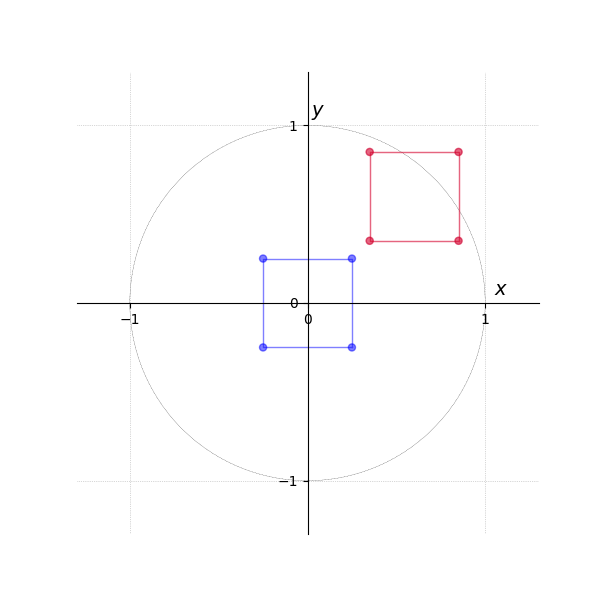
Active Transformation Example

The following example illustrates the effect of the model matrix and the rotation matrix (see Figure 2).

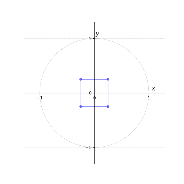
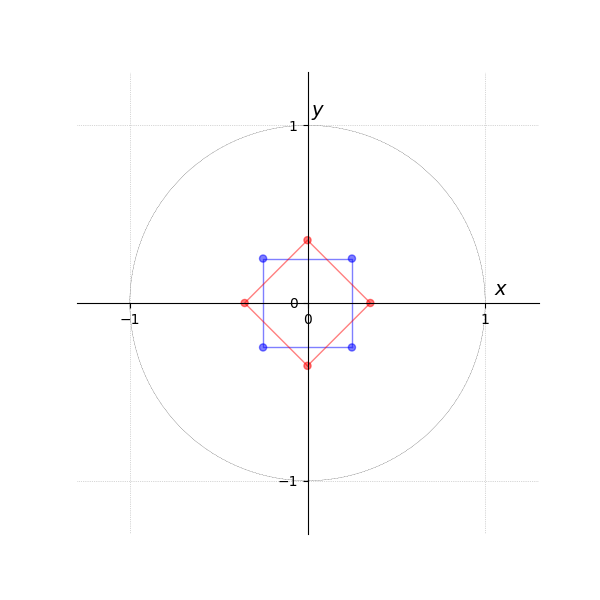
The first tab Figure 3 shows $4$ vertices in a local coordinate system.
In the next tab Figure 4, they are transformed into world coordinates via the matrix-vector multiplication $\boldsymbol{M} \vec{v}_i$.
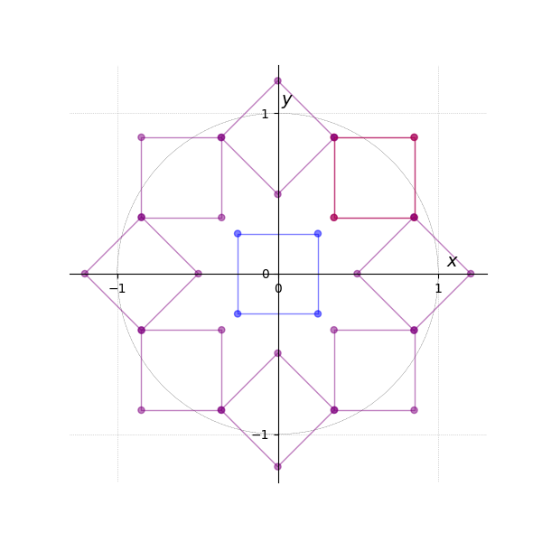
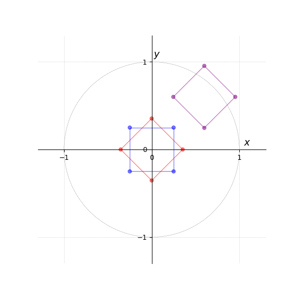
The third tab Figure 5 then generates the result of $\boldsymbol{R} \boldsymbol{M} \vec{v}_i$ eight times, with each instance rotated by an additional 45 degrees around the origin (i.e., $45\degree$, $90\degree$, $135\degree$, $180\degree$, etc.).

Translation is omitted in this example, as the transformation is relative to the origin.

Animation R*M

^{Figure 2 The animation illustrates pre-multiplying the model matrix by a rotation.}

Local Space...

^{Figure 3}

... to World Space...

^{Figure 4}

... and Rotation around Origin

^{Figure 5}

Plot-Code (Python)

import matplotlib.pyplot as plt
import numpy as np
from matplotlib.patches import Arc, FancyArrowPatch
from matplotlib.animation import FuncAnimation

fig, ax = plt.subplots(figsize=(6, 6))

def rotation(angle):
    rad=np.deg2rad(angle); cos_theta = np.cos(rad); sin_theta = np.sin(rad)
    return np.array([[cos_theta, -sin_theta, 0], [sin_theta, cos_theta, 0], [0, 0, 1]])

def draw_lines(transformed_coords, color, alpha):
    closed_coords = np.vstack([transformed_coords, transformed_coords[0]])
    ax.plot(closed_coords[:, 0], closed_coords[:, 1],  linewidth=1, color=color, alpha=alpha)

def draw_rectangle(model, vertices, color):
    for v in vertices:
        circle = plt.Circle(model @ v, 0.02, color=color[0], alpha=color[1], fill=True);
        ax.add_patch(circle);
    draw_lines(np.array([model@v for v in vertices]), color[0], color[1])

def init():
    ax.set_xlim(-1.3, 1.3); ax.set_ylim(-1.3, 1.3)
    ax.set_xticks([-1, 0, 1]); ax.set_yticks([-1, 0, 1])
    ax.set_aspect('equal'); ax.grid(True, linestyle=':', linewidth=0.5)
    for spine in ax.spines.values(): spine.set_visible(False)
    ax.spines['bottom'].set_position('zero'); ax.spines['left'].set_position('zero')
    ax.spines['bottom'].set_visible(True); ax.spines['left'].set_visible(True)
    ax.xaxis.set_ticks_position('bottom'); ax.yaxis.set_ticks_position('left')
    ax.text(1.05, 0.02, r"$x$", fontsize=14, va='bottom'); ax.text(0.02, 1.05, r"$y$", fontsize=14, ha='left')
    circle = plt.Circle((0, 0), 1, color='black', linewidth=0.2, fill=False, transform=ax.transData, linestyle='--')
    ax.add_patch(circle)

    draw_rectangle(np.identity(3), vertices, color_org)

sc=1/4 #scale distance between 0 an 1*scale
vertices = [np.array([1*sc, -1*sc, 1]), np.array([1*sc, 1*sc, 1]), np.array([-1*sc,1*sc, 1]), np.array([-1*sc,-1*sc, 1])]
model = np.array([[1, 0, 0.6],[0, 1, 0.6],[0,0,1]])
color_org=["blue", 0.5]; color_m = ["red", 0.5]; color_r=["purple", 0.5]; color_b=["black", 0.5]

def update(angle):
    ax.cla()
    init()

    R = rotation(angle)
    draw_rectangle(R@model, vertices, color_r)



angle = 0
end = 360
steps = 2

ani = FuncAnimation(fig, update, frames=list(range(0, end, steps)), interval=30)
ani.save(
    #path
    ,
    writer="pillow",
    fps=30
)

Rotating an object around its own center

If we want to use the object's own center as the pivot point for a rotation, it is sufficient to multiply the model matrix $\boldsymbol{M}$ by the rotation matrix $\boldsymbol{R}$. In this case, a separate translation to a different origin is not necessary.

The effect becomes clear when we apply the operation to a local-space vector, $\vec{v}_\text{local}$.

$$\vec{v}_\text{world} = \boldsymbol{M}\ (\boldsymbol{R}\ \vec{v}_\text{local})$$

Interpreting this from right to left as is conventional, the vector $\vec{v}_\text{local}$ is first rotated within the object's local coordinate system. Then, the model matrix is multiplied by this newly rotated local vector, transforming it into world coordinates as $\vec{v}_\text{world}$.

Since matrix multiplication is associative, we can pre-calculate a new model matrix, $\boldsymbol{M}'$, from the multiplication:

$$\boldsymbol{M'}\ = \boldsymbol{M}\ \boldsymbol{R}$$

This new matrix can then be applied to all vertices of the object to achieve the same result more efficiently.

The animation in Figure 6 shows the transformation, which is broken down in the subsequent figures. Figure Figure 7 shows the object from the previous example in its local coordinates. Figure Figure 8 then shows the rotation being applied first. Finally, Figure Figure 9 shows the multiplication by the model matrix, which transforms the already-rotated object into world coordinates.

Animation M*R

^{Figure 6 The animation shows that right-multiplying the model matrix by a rotation applies the rotation in local space (M*R).}

Local Space...

^{Figure 7}

... and Rotation around its Origin...

^{Figure 8}

... to World Space

^{Figure 9}

Plot-Code (Python)

import matplotlib.pyplot as plt
import numpy as np
from matplotlib.patches import Arc, FancyArrowPatch
from matplotlib.animation import FuncAnimation

fig, ax = plt.subplots(figsize=(6, 6))

def rotation(angle):
    rad=np.deg2rad(angle); cos_theta = np.cos(rad); sin_theta = np.sin(rad)
    return np.array([[cos_theta, -sin_theta, 0], [sin_theta, cos_theta, 0], [0, 0, 1]])

def draw_lines(transformed_coords, color, alpha):
    closed_coords = np.vstack([transformed_coords, transformed_coords[0]])
    ax.plot(closed_coords[:, 0], closed_coords[:, 1],  linewidth=1, color=color, alpha=alpha)

def draw_rectangle(model, vertices, color):
    for v in vertices:
        circle = plt.Circle(model @ v, 0.02, color=color[0], alpha=color[1], fill=True);
        ax.add_patch(circle);
    draw_lines(np.array([model@v for v in vertices]), color[0], color[1])

def init():
    ax.set_xlim(-1.3, 1.3); ax.set_ylim(-1.3, 1.3)
    ax.set_xticks([-1, 0, 1]); ax.set_yticks([-1, 0, 1])
    ax.set_aspect('equal'); ax.grid(True, linestyle=':', linewidth=0.5)
    for spine in ax.spines.values(): spine.set_visible(False)
    ax.spines['bottom'].set_position('zero'); ax.spines['left'].set_position('zero')
    ax.spines['bottom'].set_visible(True); ax.spines['left'].set_visible(True)
    ax.xaxis.set_ticks_position('bottom'); ax.yaxis.set_ticks_position('left')
    ax.text(1.05, 0.02, r"$x$", fontsize=14, va='bottom'); ax.text(0.02, 1.05, r"$y$", fontsize=14, ha='left')
    circle = plt.Circle((0, 0), 1, color='black', linewidth=0.2, fill=False, transform=ax.transData, linestyle='--')
    ax.add_patch(circle)

    draw_rectangle(np.identity(3), vertices, color_org)

sc=1/4 #scale distance between 0 an 1*scale
vertices = [np.array([1*sc, -1*sc, 1]), np.array([1*sc, 1*sc, 1]), np.array([-1*sc,1*sc, 1]), np.array([-1*sc,-1*sc, 1])]
model = np.array([[1, 0, 0.6],[0, 1, 0.6],[0,0,1]])
color_org=["blue", 0.5]; color_m = ["red", 0.5]; color_r=["purple", 0.5]; color_b=["black", 0.5]

def update(angle):
    ax.cla()
    init()

    R = rotation(angle)
    draw_rectangle(R, vertices, color_m)
    draw_rectangle(model@R, vertices, color_b)



angle = 0
end = 360
steps = 2

ani = FuncAnimation(fig, update, frames=list(range(0, end, steps)), interval=30)
ani.save(
    #path
    ,
    writer="pillow",
    fps=30
)

rotate() in glm and Unity

The glm library provides the method GLM_FUNC_DECL mat<4, 4, T, Q> glm::rotate(mat< 4, 4, T, Q > const & m, T angle, vec< 3, T, Q > const & axis)⁵. This function internally calculates a rotation matrix $R$ from the given angle and axis and returns the post-multiplied result $\boldsymbol{M} \boldsymbol{R}$. This is the standard method for applying a rotation in the local space of the input/mdoel matrix $\boldsymbol{M}$.

The Unity engine's Rotate(Vector3 eulers, Space relativeTo = Space.Self)⁶ method makes this choice explicit with an optional parameter. The default, Space.Self, performs a local rotation (equivalent to $\boldsymbol{M} \boldsymbol{R}$), while Space.World performs a world-space rotation (equivalent to $\boldsymbol{R}\ \boldsymbol{M}$).

---

Updates: 02.09.2025 initial publication

Footnotes

1. see Rotations as a Special Case of Vector Transformations ↩

2. Since $O$ ignores constant factors, we can conclude that both methods show linear complexity, $O(n)$. ↩

3. see Passive Rotation and the Composition of Transformations ↩

4. Read as an active transform, this is identical to translating the vector back after rotation was applied. ↩

5. https://glm.g-truc.net/0.9.9/api/a00247.html#gaee9e865eaa9776370996da2940873fd4, retrieved 02.09.2025 ↩

6. https://docs.unity3d.com/ScriptReference/Transform.Rotate.html, retrieved 02.09.2025 ↩