From Camera to Clip Space - Derivation of the Projection Matrices

We derive the orthographic and perspective projection matrices used in 3D computer graphics, with special emphasis on OpenGL conventions. Starting from camera-space geometry, we construct the projection that maps to clip space, explain clipping via the clip-space inequalities, and show how the subsequent perspective divide produces normalized device coordinates in the canonical view volume. Along the way, we show that affine transformations preserve parallelism. We clarify the roles of the $z$- and $w$-components: Depth in NDC arises from $z_\text{ndc} = \frac{z_\text{clip}}{w_\text{clip}}$, with $w$ carrying the perspective scaling. The result is a compact, implementation-oriented account of Field-of-View, aspect ratio and near-/far-plane parameters.

Introduction

This article describes one of the final steps in the rendering pipeline: Projection and perspective transformations.

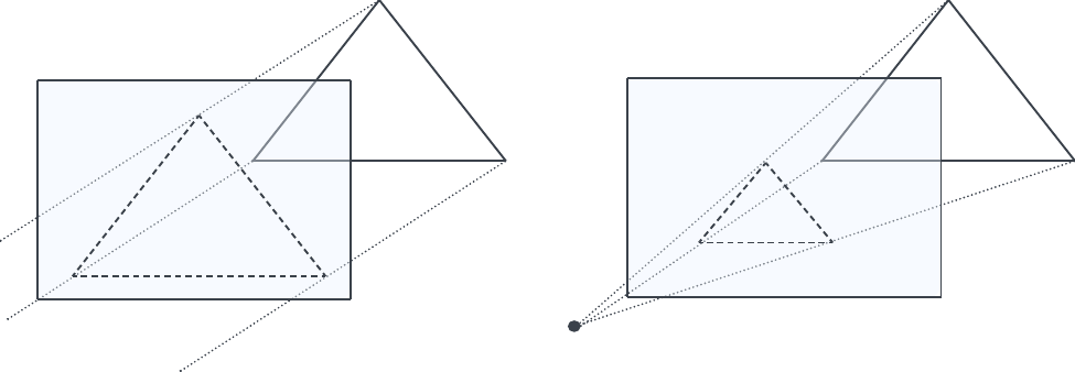
While in perspective projection all projection lines converge at a single point - producing the familiar sense of depth - in orthographic projection these lines run parallel to each other. With this projection type, parallel lines therefore remain parallel even after mapping onto the so-called unit cube.

We begin with the orthographic projection and derive a projection matrix that maps an arbitrary view volume onto the so-called unit cube. Along the way, we use figures to show how an orthographic projection affects objects we usually perceive in a perspective manner.

We then derive the perspective projection and show how choosing a near and a far viewing plane, as well as a height and a width encoded in the aspect ratio, creates a so-called view frustum that contains the objects visible to the observer, while any geometry outside of it is clipped and discarded from the rendering process.

Projection Planes

In the final steps of the rendering pipeline, the perspective divide converts clip-space coordinates to normalized device coordinates¹; the viewport transform maps them to screen space, and rasterization produces the 2D image.

Before this happens, a view matrix $\boldsymbol{M}_\text{lookAt}$ is constructed that transforms world coordinates into camera coordinates², defined by a vantage point $\text{eye}_{xyz}$, the observed point $c$ and a vector $\vec{up}$ representing the camera’s up direction at camera at $\text{eye}_{xyz}$ looking at $c$.

Transforming world coordinates into camera coordinates isn’t particularly helpful on its own. In a scene graph with hundreds of nodes, we still have to decide which ones should actually appear on screen. Even with a known viewer position and look direction, the camera is still just an idealized point; without a defined viewing volume, no geometry will be captured, and the resulting image will be empty. Conversely, knowing only the viewport's height and width defines the aspect ratio, but it tells us nothing about the field of view, depth range, or clipping planes.

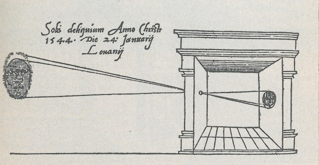
In general, the camera implicit in computing camera coordinates is a pinhole camera - an idealized model with an infinitesimally small aperture that admits rays and produces an image. We push the abstraction a step further: In computer graphics we don’t capture photons, we trace geometric lines from the scene’s vertices through the pinhole onto a projection plane. Take the camera obscura³ as a figurative example, where we place a screen behind the pinhole and the projected points meet on that plane, yielding a mirrored, upside-down image (see Figure 1).

In the following, we will define the viewing volume for both orthographic and perspective projections. We will determine the size of the projection plane and its distance from the camera and examine how these parameters determine the view frustum, which specifies which objects in the scene are ultimately rendered.

^{Figure 1 First published picture of camera obscura in Gemma Frisius' 1545 book De Radio Astronomica et Geometrica. (Source: Wikipedia)}

Excursus: View Space, Clip Space, the Canonical View Volume and NDCs

In the following, we will give a brief introduction to clipping, which is a process that discards geometry outside of a view volume. In short, primitives removed during clipping will not be part of the Canonical View Volume which contains all necessary geometry passed on to the final rasterization and on-screen display stages of the rendering pipeline.

Clipping is done by OpenGL with the help of the homogeneous coordinate component $w$. The following introduces the process with the help of orthographic projection, but it can be applied analogously with perspective projection, as we will see later.

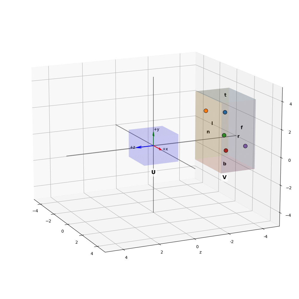
In camera space, the six planes $l, r, b, t, n, f$ of a view volume $\boldsymbol{V}$ specify the clipping planes (see Figure 2). Roughly speaking, all vertices within this view volume $\boldsymbol{V}$ are considered to be preserved for rendering.

^{Figure 2 Visualization of the unit cube U as the target NDC space and a generic view volume V and its contents to be projected into U after the perspective divide. The illustration shows the camera space of the scene.}

After multiplying a vertex with the projection matrix, the vertex shader's homogeneous coordinate

gl_Position = $(x, y, z, w)$

is in clip space⁴.

OpenGL then performs clipping of the primitives against the inequalities [📖KSS17, Figure 5.2, 201]⁵

$$\begin{alignat*}{3} & -w \leq x \leq w \\ \land \quad & -w \leq y \leq w \\ \land \quad & -w \leq z \leq w \end{alignat*}$$

Primitives outside clip space are discarded, while the visible portion of intersecting primitives is rasterized [📖SWH15, 2 96ff.].

Once clipping has finished, the clip coordinates are mapped to Normalized Device Coordinates by the perspective divide

$$(x_\text{ndc}, y_\text{ndc}, z_\text{ndc}) = (\frac{x}{w}, \frac{y}{w}, \frac{z}{w})$$

This yields the coordinates within the canonical view volume. Since every surviving clip coordinate $(x, y, z, w)$ satisfies the clipping inequalities (e.g., $-w \leq x \leq w$), every component of the resulting NDC coordinate is guaranteed to lie in the interval [-1, 1]⁶.

The Canonical Unit Cube, or canonical view volume [📖RTR, 94], defined by the interval $[−1,1]$⁷ on all three axes, is the space for Normalized Device Coordinates in OpenGL.

In the rendering pipeline, NDCs are produced by applying the perspective divide $(\frac{x}{w}, \frac{y}{w},\frac{z}{w})$ to the clip space coordinates that result from the projection transform. With orthographic projection, it follows that $w=1$. The coordinates resulting from this normalization step are then mapped to the user's specific device resolution (see [📖LGK23, Fig. 5.36, 181]).

When using orthographic projection, the clip space falls together with the NDCs, as the perspective division by the fourth homogeneous $w$-coordinate is applied, but does not change the $x,y,z$-coordinates (see [📖SWH15, 72]).

Defining the Canonical View Volume in OpenGL

Let $(x, y, z)$ be a point in view space. This is in homogeneous coordinates

$$(x, y, z, 1)$$

After transforming into clip space, the point is mapped to

$$(x_\text{clip}, y_\text{clip}, z_\text{clip}, w_\text{clip}), \ w_\text{clip} \ne 0$$

Let $|x_\text{clip}| \le |w_\text{clip}|$. Then, the following holds:

$$|x_\text{clip}| \le |w_\text{clip}| \Leftrightarrow |\frac{x_\text{clip}}{w_\text{clip}}| \le 1$$

Obviously, since

$$|x_\text{ndc}| = |\frac{x_\text{clip}}{w_\text{clip}}| \le 1$$

the inequality

$$-w_\text{clip} \leq x_\text{clip} \leq w_\text{clip} \Leftrightarrow -1 \leq x_\text{ndc} \leq 1$$

holds.

Applying the same premise and same logic to $y_\text{clip}, z_\text{clip}$ shows that $(x_\text{ndc}, y_\text{ndc}, z_\text{ndc})$ is in $[-1, 1]^3$.

Therefor, any point that is not clipped before the perspective divide must satisfy the inequalities

$$\begin{alignat*}{3} & -w_\text{clip} \leq x_\text{clip} \leq w_\text{clip} \\ \land \quad & -w_\text{clip} \leq y_\text{clip} \leq w_\text{clip} \\ \land \quad & -w_\text{clip} \leq z_\text{clip} \leq w_\text{clip} \end{alignat*}$$

which yields a point in NDC in the Canonical View Volume in OpenGL⁸ that satisfies

$$\begin{alignat*}{3} & -1 \leq x_\text{ndc} \leq 1 \\ \land \quad & -1 \leq y_\text{ndc} \leq 1 \\ \land \quad & -1 \leq z_\text{ndc} \leq 1 \end{alignat*}$$

$\Box$

Orthographic Projection

When we apply orthographic projection, points are projected onto an arbitrary plane.

Visually, it appears as if we are reducing the vector space by one dimension. A key property is that parallel lines remain parallel, regardless of the camera's orientation, and the perspective component is eliminated.

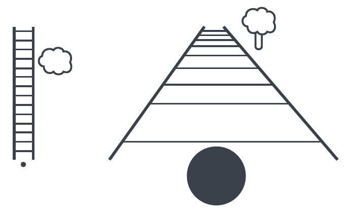
To explain this intuitive sense of depth and the apparent contradiction with parallel lines, the example of railroad tracks is often used: While we can assume that railroad tracks are parallel not only at the observer's standpoint but also a kilometer in the distance, the effect of depth makes it seem as though the tracks converge at a single point, known as the vanishing point (see Figure Figure 6).

^{Figure 6 The left side shows an orthographic (top-down) view of a spectator and railroad tracks. In this objective view, parallel lines remain parallel. The right side shows a perspective view from the spectator's vantage point. Here, the parallel tracks recede into the distance, appearing to converge at a vanishing point and demonstrating how our eyes perceive depth. (Source: own)}

For eliminating the z-component of any given $\vec{v} \in \mathbb{R}^3$, we can use the following matrix:

$$\begin{pmatrix} 1 & 0 & 0 & 0\\ 0 & 1 & 0 & 0\\ 0 & 0 & 0 & 0\\ 0 & 0 & 0 & 1\\ \end{pmatrix}$$

From this matrix form it immediately follows that any homogenous vector $\vec{v} = (x, y, z, 1)^T$ multiplied with this matrix yields a vector $\vec{v'}$ with its z-component set to $0$:

$$\begin{pmatrix} 1 & 0 & 0 & 0\\ 0 & 1 & 0 & 0\\ 0 & 0 & 0 & 0\\ 0 & 0 & 0 & 1\\ \end{pmatrix} \begin{pmatrix} x \\ y \\ z \\ 1 \end{pmatrix} = \begin{pmatrix} x \\ y \\ 0 \\ 1 \end{pmatrix}$$

To project onto an arbitrary z-plane, we use the z-component of the 4 column in the matrix and construct a transformation matrix

$$\boldsymbol{M_o} = \begin{pmatrix} 1 & 0 & 0 & 0\\ 0 & 1 & 0 & 0\\ 0 & 0 & 0 & z_p\\ 0 & 0 & 0 & 1\\ \end{pmatrix}$$

This gives us

$$\boldsymbol{M_o} \begin{pmatrix} x \\ y \\ z \\ 1 \end{pmatrix} = \begin{pmatrix} (1, 0, 0, 0)^T \cdot (x, y, z, 1)^T \\ (0, 1, 0, 0)^T \cdot (x, y, z, 1)^T \\ (0, 0, 0, z_p)^T \cdot (x, y, z, 1)^T \\ (0, 0, 0, 1)^T \cdot (x, y, z, 1)^T \end{pmatrix} = \begin{pmatrix} x \\ y \\ z_p \\ 1 \end{pmatrix}$$

We can easily derive that any vector computed by this must be perpendicular to the plane given by the vectors $(x, 0, 0)^T$ and $(0, y, 0)^T$, since their crossproduct yields

$$\begin{pmatrix} x \\ 0 \\ 0 \end{pmatrix} \times \begin{pmatrix} 0 \\ y \\ 0 \end{pmatrix} = \begin{pmatrix} 0 \\ 0 \\ xy \end{pmatrix}$$

which is a vector $\vec{xy}$ with $|\vec{xy}| = sin(\theta) |\vec{x}| |\vec{y}|$.

It is easily shown that this vector is parallel to $(0, 0, z_p)^T$ since

$$\begin{pmatrix} 0 \\ 0 \\ xy \end{pmatrix} \times \begin{pmatrix} 0 \\ 0 \\ z_p \end{pmatrix} = \begin{pmatrix} 0 \\ 0 \\ 0 \end{pmatrix}$$

The effect of projecting the points of a (wireframed) cube is shown in the animations Figure 3, Figure 5, Figure 4.

^{Figure 3 An isometric view showing a cube being orthographically projected onto the highlighted plane at z=-4.}

^{Figure 3 Here, the same scene is rendered with a direct orthographic view, eliminating all perspective. This illustrates the final 2D image as it would appear on a screen if the camera was directly in front of the cube.}

^{Figure 3 Instead of rendering the entire scene orthographically, we first project it onto z=-4 and then visualize this 2D result with a perspective camera on the negative z-axis, an optical axis orthogonal to the plane.}

Plot-Code (Python)

import numpy as np
import matplotlib.pyplot as plt
from mpl_toolkits.mplot3d import Axes3D  # noqa: F401
from mpl_toolkits.mplot3d.art3d import Poly3DCollection
import math
from matplotlib.animation import FuncAnimation

# Convention: x -> right, y -> up, z -> toward viewer. (rhs)

def rotate(theta, n, v, pivot):
    v = v-pivot
    theta = theta * math.pi/180
    vn = v / np.linalg.norm(v)
    nn = n / np.linalg.norm(n)
    vpar = np.dot(nn, v) * nn
    vperp = v - vpar

    return vpar + (np.cos(theta) * (vperp)) + (np.sin(theta) * np.cross(nn, v)) + pivot

def to_matplotlib(xu, yu, zu):
    return xu, zu, yu

xr = (-5, 5)
yr = (-5, 5)
zr = (5, -5)

fig = plt.figure(figsize=(10, 10))
ax = fig.add_subplot(111, projection='3d')
# set to ortho for orthographic projection of the plot
# ax.set_proj_type('ortho')

def init():

    ax.set_xlim(*xr)
    ax.set_ylim(-zr[0], -zr[1])
    ax.set_zlim(*yr)

    z_plane = -4.0
    x = np.linspace(xr[0], xr[1], 40)
    y = np.linspace(yr[0], yr[1], 40)
    Xg, Yg = np.meshgrid(x, y)
    Xm, Ym, Zm = to_matplotlib(Xg, Yg, z_plane)

    ax.plot_surface(Xm, Ym, Zm, alpha=0.15, linewidth=0, antialiased=True)

    # Wireframe
    xw = np.linspace(xr[0], xr[1], 12)
    yw = np.linspace(yr[0], yr[1], 12)
    Xw, Yw = np.meshgrid(xw, yw)
    Xm_w, Ym_w, Zm_w = to_matplotlib(Xw, Yw, z_plane)
    ax.plot_wireframe(Xm_w, Ym_w, Zm_w, rstride=1, cstride=1, linewidth=0.5)

    # Coordinate axes in USER coordinates
    Xline = np.linspace(xr[0], xr[1], 2)
    Xm_ax, Ym_ax, Zm_ax = to_matplotlib(Xline, 0*Xline, 0*Xline)
    ax.plot(Xm_ax, Ym_ax, Zm_ax,  color="black", alpha=0.5)

    Yline = np.linspace(yr[0], yr[1], 2)
    Xm_ay, Ym_ay, Zm_ay = to_matplotlib(0*Yline, Yline, 0*Yline)
    ax.plot(Xm_ay, Ym_ay, Zm_ay, color="black", alpha=0.5)

    Zline = np.linspace(zr[0], zr[1], 2)
    Xm_az, Ym_az, Zm_az = to_matplotlib(0*Zline, 0*Zline, Zline)
    ax.plot(Xm_az, Ym_az, Zm_az,  color="black", alpha=0.5)

    arrow_len = 2.0
    # +x
    dx, dy, dz = to_matplotlib(1, 0, 0)
    ax.quiver(0, 0, 0, dx, dy, dz, color="red", length=arrow_len, normalize=True)
    # +y
    dx, dy, dz = to_matplotlib(0, 1, 0)
    ax.quiver(0, 0, 0, dx, dy, dz, color="green", length=arrow_len, normalize=True)
    # +z
    dx, dy, dz = to_matplotlib(0, 0, 1)
    ax.quiver(0, 0, 0, dx, dy, dz, color="blue", length=arrow_len, normalize=True)

    ax.text(*to_matplotlib(arrow_len*1.1, 0, 0), "+x")
    ax.text(*to_matplotlib(0, arrow_len*1.1, 0), "+y")
    ax.text(*to_matplotlib(0, 0, arrow_len*1.1), "+z")

    # Change perspective here (world cam)
    ax.view_init(elev=15, azim=-25)
    #ax.view_init(elev=0, azim=-90)

def rays(points, z_target):
        colors = [
            '#FF0000',
            '#0000FF',
            '#00FF00',
            '#FF8000',
            '#8000FF',
            '#00FFFF',
            '#FF00FF',
            '#FFFF00'
        ]

        i=0
        for p in points:
            # p is in USER-Coordinates
            x, y, z = to_matplotlib(
                [p[0], p[0]],
                [p[1], p[1]],
                [p[2], z_target],  # orthogonal projection on z = z_target
            )

            ax.plot(x, y, z, color=colors[i], alpha=0.5)
            i+=1

def update(theta):
    ax.cla()
    init()

    # Back face center and parameters in USER coordinates
    cx, cy, zb = 4.0, 3.5, 1.0
    s = 1.0      # side length
    h = s / 2.0
    zf = zb + s  # front face z

    pivot = np.array([cx, cy, (zb + zf)/2.0])

    axis= np.array([0, 1, 0])

    # Back face corners (on z = zb)
    bl_b = rotate(theta, axis, np.array([cx - h, cy - h, zb]), pivot)  # bottom-left
    br_b = rotate(theta, axis, np.array([cx + h, cy - h, zb]), pivot)  # bottom-right
    tr_b = rotate(theta, axis, np.array([cx + h, cy + h, zb]), pivot)  # top-right
    tl_b = rotate(theta, axis, np.array([cx - h, cy + h, zb]), pivot)  # top-left

    # Front face corners (on z = zf)
    bl_f = rotate(theta, axis, np.array([cx - h, cy - h, zf]), pivot)
    br_f = rotate(theta, axis, np.array([cx + h, cy - h, zf]), pivot)
    tr_f = rotate(theta, axis, np.array([cx + h, cy + h, zf]), pivot)
    tl_f = rotate(theta, axis, np.array([cx - h, cy + h, zf]), pivot)

    z_target = -4

    rays([bl_b, br_b, tr_b, tl_b, bl_f, br_f, tr_f, tl_f], z_target);

    faces_user = [
        [bl_b, br_b, br_f, bl_f],  # bottom side (y = cy - h)
        [br_b, tr_b, tr_f, br_f],  # right side  (x = cx + h)
        [tr_b, tl_b, tl_f, tr_f],  # top side    (y = cy + h)
        [tl_b, bl_b, bl_f, tl_f],  # left side   (x = cx - h)
    ]

    faces_mat = [[to_matplotlib(*p) for p in face] for face in faces_user]

    # from faces_user ...
    proj_faces_user = [[[p[0], p[1], z_target] for p in face] for face in faces_user]

    # ... to projected coordinates (with y/z swap)
    proj_faces = [[to_matplotlib(*p) for p in face] for face in proj_faces_user]

    for face in faces_mat:
        xs = [p[0] for p in face] + [face[0][0]]
        ys = [p[1] for p in face] + [face[0][1]]
        zs = [p[2] for p in face] + [face[0][2]]
        ax.plot(xs, ys, zs, linewidth=1.25, color="purple")

    for face in proj_faces:
        xs = [p[0] for p in face] + [face[0][0]]
        ys = [p[1] for p in face] + [face[0][1]]
        zs = [p[2] for p in face] + [face[0][2]]
        ax.plot(xs, ys, zs, linewidth=1.25, color="purple")


    theta += 5

end = 180
steps = 2
theta = 0


ani = FuncAnimation(fig, update, frames=list(range(0, end, steps)), interval=30, init_func=init)
#foo=ani.save(path/filename.gif, writer="pillow", fps=30)
init()
plt.tight_layout()

plt.show()

Affine Transformation

The statement that two parallel vectors $\vec{p}, \vec{q}$ remain parallel after an orthographic projection is applied is a fundamental property of an affine transformation [📖VB15, 118].

An affine transformation $\boldsymbol{T}$ is a transformation of the form

$$\vec{v'} = \boldsymbol{T}(\vec{v}) = \boldsymbol{L}(\vec{v}) + \vec{x}$$

where $\boldsymbol{L}$ is a linear transformation. Hence, an affine transformaton is simply a linear transformation to which a translation is applied.

Intuitively, we can see that this statement holds. Given two parallel vectors:

$$\vec{p} = \begin{pmatrix}x \\ y \\ z \end{pmatrix}, \ \vec{q} = \begin{pmatrix}x' \\ y' \\ z' \end{pmatrix}$$

Their cross product is the zero vector

$$\vec{p} \times \vec{q} = (x, y, z)^T \times (x', y', z')^T = (yz' - zy', zx' - xz', xy' - x'y) = \vec{0}$$

which yields three initial conditions:

$$yz' - zy' = 0 \Leftrightarrow yz' = zy' \\ zx' - xz' = 0 \Leftrightarrow zx' = xz' \\ xy' - x'y = 0 \Leftrightarrow xy' = x'y \\$$

Obviously, removing the z component from $\vec{p}$ and $\vec{q}$ preserves the parallelism for the $xy$-plane, as the third component of the cross product is still zero:

$$\begin{pmatrix} x \\ y \\ 0 \end{pmatrix} \times \begin{pmatrix} x' \\ y' \\ 0 \end{pmatrix} = \begin{pmatrix} 0 \\ 0 \\ xy' - x'y = 0 \end{pmatrix} = \vec{0}$$

Our intution tells us that since these new vectors are parallel, translating both by an equal amount in the same direction will not change their parallelism. Therefor, adding the same z-component $(0, 0, z_p)^T$ to both vectors yields to parallel vectors

$$\vec{p'} = \begin{pmatrix}x \\ y\\ z_p \end{pmatrix}, \vec{q'} = \begin{pmatrix}x' \\ y'\\ z_p \end{pmatrix}$$

This intuition can be formalized using the definition of an affine transformation. We can write our orthographic projection Matrix $\boldsymbol{M_o}$ as an affine transformation $\boldsymbol{T}$ consisting of the sum of a linear combination

$$\boldsymbol{L}(\vec{v}) = \begin{pmatrix} 1 & 0 & 0 \\ 0 & 1 & 0 \\ 0 & 0 &0 \end{pmatrix} \begin{pmatrix}v_0 \\v_1 \\v_2 \end{pmatrix} = \begin{pmatrix} v_0 \\ v_1 \\ 0 \end{pmatrix}$$

and a translation vector $\vec{z_p}$. That affine transformations preserve parallelism will be shown for the general case in the next section.

Proof that Affine Transformations preserve Parallelism

Proof

Let $\boldsymbol{T}$ be an affine transformation

$$\boldsymbol{T}(\vec{v}) = \boldsymbol{L}(\vec{v}) + \vec{z_p}$$

Let's define two lines $p_l$, $q_l$ with direction vectors $\vec{p} = P_2 - P_1$ and $\vec{q} = Q_2 - Q_1$, where $P_i, Q_i$ are points on the respective lines.

Since the lines are parallel, we can write $\vec{p}$ as the scaled version of $\vec{q}$

$$\vec{p} = k \vec{q},\ k \in \mathbb{R}$$

Applying the affine transformation to the points $P_1$ and $P_2$ yields a new vector with direction $\vec{p}'$:

$$\begin{alignat*}{3} \vec{p'} &= T (P_2) - T(P_1) \\ &= (\boldsymbol{L}(P_2) + \vec{z_p}) - (\boldsymbol{L}(P_1) + \vec{z_p})\\ &= \boldsymbol{L}(P_2) - \boldsymbol{L}(P_1) \end{alignat*}$$

Since $\boldsymbol{L}$ is a linear transformation, we can simplify this to

$$\vec{p'} = \boldsymbol{L}(P_2) - \boldsymbol{L}(P_1) = \boldsymbol{L}(P_2 - P_1) = \boldsymbol{L}(\vec{p})$$

This shows that the new direction vector is the result of applying the linear part of the transformation to the original direction vector. Applying the same computation to $q_l$ gives us

$$\vec{q'} = \boldsymbol{L}(Q_2) - \boldsymbol{L}(Q_1) = \boldsymbol{L}(Q_2 - Q_1) = \boldsymbol{L}(\vec{q})$$

Since we know $\vec{p} = k \vec{q}$, we can therefore conclude:

$$\vec{p'} = \boldsymbol{L}(\vec{p}) = \boldsymbol{L}(k \vec{q}) = k \boldsymbol{L}(\vec{q}) = k \vec{q'}$$

Hence, $\vec{p}'$ is $\vec{q}'$ scaled by $k$, which shows that they are parallel. This proves that any affine transformation $\boldsymbol{T}$ preserves parallelism. $\Box$

Deriving the Orthographic Projection Matrix

In the following, we will derive the orthographic projection matrix required to map an arbitrary cubic volume $\boldsymbol{V}$ from view space coordinates⁹ to the canonical view volume $\boldsymbol{U}$.

We begin with defining the coordinates of the Volume $\boldsymbol{V}$ to be projected (see Figure 2):

$$\begin{alignat*}{3} l \qquad &(\text{left})\\ r \qquad &(\text{right})\\ b \qquad &(\text{bottom})\\ t \qquad &(\text{top})\\ n \qquad &(\text{near})\\ f \qquad &(\text{far}) \end{alignat*}$$

The naming convention applies after the transformations to camera space. In this space, the camera is located at the origin $(0, 0, 0)$, looking down the negative $z$-axis. $\boldsymbol{V}$ is defined by coordinates relative to the z-axis. Figure 2 shows therefore a representation of camera space.

Note that $n$, $f$ represent positive distances to the near and far clipping planes. By definition, the near plane is closer to the origin, so $n < f$.

However, in camera space where the view direction is along the negative $z$-axis, these values correspond to negative coordinates. The near plane is located at

$$z_\text{near} = -n$$

The far plane is located at

$$z_\text{far} = -f$$

Therefore, the following holds:

$$z_\text{near} > z_\text{far}$$

When deriving the coordinates for the canonical view volume, we adopt standard OpenGL convention in form of a left handed coordinate system, that is, the view direction is along the positive instead of the negative $z$-axis. For our case this means that we have to mirror the $z$-axis at the origin, which will be considered by using a negative $z$-component in the following orthographic projection matrix (see [📖RTR, 95]).

We will first examine the requirements for the affine transformation. Since all vertices of V must fit into the unit cube $[−1,1]^3$, which - probably unlike $\boldsymbol{V}$ - is located at the origin, a translation and a scaling are necessary. Thus, we can directly define a transformation matrix of the form

$$\begin{pmatrix} \boldsymbol{S} & \vec{t} \\ 0 & 1 \end{pmatrix}$$

where $\boldsymbol{S}$ is the $3 \times 3$ scaling matrix and $\vec{t}$ is the translation vector.

We thus obtain the affine transformation that, when multiplied by an arbitrary vertex $(x, y, z, 1)^T$, transforms it into the canonical view volume:

$$\begin{pmatrix} a_x & 0 & 0 & b_x \\ 0 & a_y & 0 & b_y \\ 0 & 0 & -a_z & b_z \\ 0 & 0 & 0 & 1 \\ \end{pmatrix} \begin{pmatrix} x \\ y\\ z \\ 1 \end{pmatrix} = \begin{pmatrix} a_xx+b_x \\ a_yy+b_y\\ -a_zz+b_z \\ 1 \end{pmatrix}$$

Here, we have negated the $z$-component, as we must mirror the $z$-axis (see above).

From this, we can derive a system of linear equations for which the following conditions must be met:

$$\begin{alignat*}{3} a_xl + b_x = -1 \ &\land a_xr + b_x = 1 && \qquad (\text{x-Axis})\\ a_yb + b_y = -1 \ &\land a_yt + b_y = 1 && \qquad (\text{y-Axis}) \\ -a_z\cdot (-n) + b_z = -1 \ &\land -a_z\cdot (-f) + b_z = 1 && \qquad (\text{z-Axis}) \\ \end{alignat*}$$

We explicitly use $-n$ and $-f$ here because after the view transformation, the near and far values are given to us as positive distances. For the correct derivation, they must therefore be re-inserted as negative values.

Solving for $l$ and $r$, respectively, yields:

$$\begin{alignat*}{3} a_xl + b_x = -1 & \Leftrightarrow b_x = -1 - a_xl\\ \\ a_xr + b_x = 1 & \Leftrightarrow b_x = 1 - a_xr \end{alignat*}$$

Substituting $b_x$ with $-1 - a_xl$ gives us

$$\begin{alignat*}{3} a_xr -1 - a_xl = 1 & \Leftrightarrow a_xr - a_xl = 2\\ \\ & \Leftrightarrow a_x = \frac{2}{r - l} \end{alignat*}$$

Solving analogously for $a_y$ and $a_z$, we obtain

$$\begin{alignat*}{3} a_x &= \frac{2}{r - l}\\ \\ a_y &= \frac{2}{t - b}\\ \\ a_z &= \frac{2}{f - n} \end{alignat*}$$

We can now solve for $b_x, b_y, b_z$. We obtain

$$\begin{alignat*}{3} b_x &= -\frac{r+l}{r - l}\\ \\ b_y &= -\frac{t+b}{t - b}\\ \\ b_z &= -\frac{f+n}{f - n} \end{alignat*}$$

Which results in the orthographic projection matrix

$$\boldsymbol{T} = \begin{pmatrix} \frac{2}{r - l} & 0 & 0 & -\frac{r+l}{r - l} \\ 0 & \frac{2}{t - b} & 0 & -\frac{t+b}{t - b} \\ 0 & 0 & -\frac{2}{f - n} & -\frac{f+n}{f - n} \\ 0 & 0 & 0 & 1 \\ \end{pmatrix}$$

Where is the Projection Plane?

The near plane is called the "image plane" by the Red Book: It's the plane closest to the eye and perpendicular to the line of sight (see [📖KSS17, 902]). Lehn et al. equally describe the projection plane identical to the near clipping plane [📖LGK23, 166].
As such, with orthographic projection, rays from vertices of the view volume in camera space intersect the projection plane - that is usually between the near and far plane - perpendicularly. Then, after the orthographic projection is applied, clip space coordinates are transformed into the Canonical View Volume and NDCs, where the perpendicular relationship is preserved due to the parallelism-preserving properties of affine transformations. Consequently, the projection rays remain perpendicular to any $xy$-plane at $z \in [-1, 1]$ in NDC space. Think of the projection plane at $z=0$ in the final image on screen, where the $z$-component of the NDC coordinates is only used for depth testing.

Proof that (l, b, -n, 1) maps (-1, -1, -1, 1)

Let $\vec{v}$ be the homogeneous coordinate $(l, b, -n, 1)$ with $l, b, n \in \mathbb{R}$ (view space coordinates). We can then solve with $\boldsymbol{T}\vec{v}$ for

$$\begin{pmatrix} \frac{2}{r - l} & 0 & 0 & -\frac{r+l}{r - l} \\ 0 & \frac{2}{t - b} & 0 & -\frac{t+b}{t - b} \\ 0 & 0 & -\frac{2}{f - n} & -\frac{f+n}{f - n} \\ 0 & 0 & 0 & 1 \\ \end{pmatrix} \begin{pmatrix} l \\ b \\ -n \\ 1 \end{pmatrix} = \begin{pmatrix} \frac{2l}{r - l} -\frac{r+l}{r - l} \\ \frac{2b}{t - b} -\frac{t+b}{t - b} \\ -\frac{-2n}{f - n} -\frac{f+n}{f - n} \\ 1 \end{pmatrix} = \begin{pmatrix} -\frac{r - l}{r - l} \\ -\frac{t-b}{t - b} \\ -\frac{f-n}{f - n} \\ 1 \end{pmatrix} = \begin{pmatrix} -1 \\ -1 \\ -1 \\ 1 \end{pmatrix}$$

$\Box$

We can analogously show that $(r, t, -f, 1)$ maps $(1, 1, 1, 1)$.

Perspective Projection

In orthographic projection, the viewer is theoretically at an infinite distance from the projection surface, so that the rays from the impact points of the projected geometry, which are perpendicular to the projection surface, only converge at an infinite distance. For this reason, the effect of depth is absent, because objects farther back in the view volume are mapped exactly onto the projection surface and therefore correspond to their actual dimensions in space¹⁰.

Perspective projection, on the other hand, uses the camera position as a center of projection where all projection rays converge, forming a pyramid. The near and far planes clip this pyramid, defining a truncated pyramid known as the view frustum. Due to this pyramid shape, the near plane is necessarily smaller than the far plane - a key difference from orthographic projection, where the view volume is in a rectangular shape (see Figure 7).

^{Figure 7 Illustration of Orthographic (left) and Perspective (right) Projection. (Source: Based on [LGK23, Fig. 5.25, 168])}

Even with a View Frustum, the near and far planes are understood as clipping planes. However, the dimension of the far plane is also determined by another parameter, Field-of-View (fov), as we will see in the following: This parameter describes the viewer's field of vision, i.e., the area that the viewer can capture.

If the fov is correspondingly large, this affects the dimension of the far plane, and thus the volume of the View Frustum becomes larger, and thus also the amount of objects that can be captured and projected onto the near plane. This affects the size of the projections - intuitively, more objects must be projected onto the limited surface of the near plane. As a result, individual objects must appear smaller to fit within the view.

The distance of the camera from the object also has a direct effect on its projected size.

However, the distance of the near plane from the projection center has no effect on the size of displayed objects, as long as the fov remains constant. We will come back to this in a later section.

We will also see that with perspective projection, after the conversion to NDC, the property that parallel lines are preserved no longer holds for the general case due to the perspective division.

Deriving the Perspective Projection Matrix

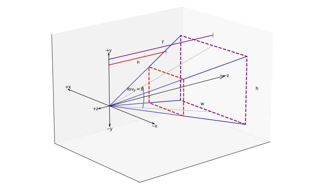
Figure 8 shows the geometric relationships between the parameters described in the introductory text. Besides the already mentioned fov $\theta$, the aspect ratio is also shown, which describes the ratio between the width ($w$) and height ($h$) of the projection surface. In the following, we will first assume an aspect ratio of 1:1 and thus an equal $\theta$ in both the vertical and horizontal directions, before we use the field of view only for the vertical direction, while the horizontal is determined by the vertical field-of-view (fovy) and the aspect ratio, as is common in OpenGL.

^{Figure 8 Camera-space perspective frustum. The eye is at the origin and looks down the negative z-axis. Width w and height h encode the aspect ratio w/h. (Source: Based on [HDMS+14, Figure 13.4, 303])}

A simple perspective projection

As with orthographic projection, we can first consider the simple case of projecting onto the $xy$-plane at $z_p$.

The projection of the point $(x, y, z)$ onto the plane $z = z_p$ to $(x', y', z_p)$ can be computed as follows:

According to the similar triangles theorem, the following holds:

$$\frac{y'}{z_p} = \frac{y}{z} \qquad (= \tan(\alpha_y))$$

From this we obtain

$$y' = \frac{yz_p}{z}$$

Analogously for $x$:

$$\frac{x'}{z_p} = \frac{x}{z} \Leftrightarrow x' = \frac{xz_p}{z} \qquad (= \tan(\alpha_x))$$

From this, a transformation matrix can be derived that maps the point $(x, y, z)$ to the point $(x', y', z_p)$:

$$\begin{pmatrix} x z_p \\ y z_p \\ z z_p \\ z \end{pmatrix} = \begin{pmatrix} z_p & 0 & 0 & 0 \\ 0 & z_p & 0 & 0 \\ 0 & 0 & z_p & 0 \\ 0 & 0 & 1 & 0 \end{pmatrix} \begin{pmatrix} x \\ y \\ z \\ 1 \end{pmatrix}$$

After the perspective division by the $w$-component of the resulting homogeneous vector, we obtain:

$$\begin{pmatrix} \frac{x z_p}{z} \\ \frac{y z_p}{z} \\ \frac{z z_p}{z} \\ \frac{z}{z} \end{pmatrix}$$

and thus the homogeneous vector that represents $(x', y', z_p)$:

$$\begin{pmatrix} \frac{x z_p}{z} \\ \frac{y z_p}{z} \\ \frac{z z_p}{z} \\ \frac{z}{z} \end{pmatrix} = \begin{pmatrix} x' \\ y' \\ z_p \\ 1 \end{pmatrix}$$

Perspective Division

As Lehn et al. note, the final row of the matrix deviates from the $(0, 0, 0, 1)$ form seen in affine transformation matrices so far. Consequently, a vertex transformed by this matrix results in a clip-space coordinate that is not yet normalized, which is achieved by the perspective division [📖LGK23, 176]. (After this division, the fourth component is discarded, yielding the final coordinates in NDC.)

The matrix notation follows Lehn et al. [📖LGK23, 171]. An alternative form is presented by Akenine-Möller et al. [📖RTR, 96]:

$$\begin{pmatrix} 1 & 0 & 0 & 0 \\ 0 & 1 & 0 & 0 \\ 0 & 0 & 1 & 0 \\ 0 & 0 & -\frac{1}{z_p} & 0 \end{pmatrix}$$

The term in the fourth row is set to $-\frac{1}{z_p}$, with $z_p$ being the absolute distance to the projection plane on the negative $z$-axis. This accounts for the convention of looking down the negative $z$-axis in view space and the axis-flip when converting to clip space, as was established during the derivation of the orthographic projection matrix. It is easy to show that both matrices yield the same results when both consider the axis flip.

Perspective Projection Matrix

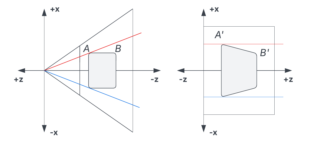
Functions like glm::perspective¹¹ create a projection matrix that transform view space coordinates into clip space. The subsequent perspective divide, a step automatically handled by OpenGL, converts these coordinates into NDC. This process creates the illusion of perspective, as dividing by the $w$-component scales each vertex's position relative to its distance from the camera.

Unlike an orthographic projection, the $w$ component od the resulting clip-space coordinate is not $1$. Instead, it is proportional to the absolute depth of the vertex in view space ($z_\text{view}$). During the perspective divide, a larger $w$ for a vertex farther away from the camera result in smaller NDC coordinates, causing the object to appear smaller on screen. Conversely, smaller $w$ contribute to larger NDC coordinates. The effect is illustrated in Figure 9.

^{Figure 9 The way the projection lines are spreading out from a single point causes lines closer to the near plane to be magnified, while correspondingly compressing lines closer to the far plane. (Source: Based on [HDMS+14, Figure 13.10, 308])}

Vanishing point and why parallelism is lost

The vanishing point, characteristic for depth-rendered illustrations, is the finite point on the screen where parallel lines appear to converge. In 3D graphics, this effect is a direct result of the perspective divide.

As derived previously, a simple perspective projection maps a point $(x,y,z)$ to the following coordinates on the projection plane after the perspective divide:

$$\begin{pmatrix} \frac{x z_p}{z}\\ \frac{y z_p}{z}\\ - z_p \end{pmatrix}$$

To find the vanishing point for lines parallel to the $z$-axis, we can examine the limit of this point as it moves to infinity:

$$\underset{z \mapsto \infty}{\lim}\begin{pmatrix} \frac{x z_p}{z}\\ \frac{y z_p}{z}\\ - z_p \end{pmatrix} = \begin{pmatrix}0 \\ 0 \\ - z_p \end{pmatrix}$$

This shows that regardless of their initial $x$ and $y$ values, all lines parallel to the $z$-axis converge to the single point

$$\begin{pmatrix} 0\\ 0\\ -z_p \end{pmatrix}$$

on the projection plane. This point of convergence is the vanishing point¹² (see [📖LGK23, 172]).

To construct a perspective projection matrix, the following parameters define the view frustum:

• Vertical Field of View $\text{fovy}$: The vertical field of view, denoted as $\theta$.
• Aspect ratio $r$: The ratio of the viewport's width $w$ and its height $h$, $r = \frac{w}{h}$.
• Near plane distane $n$: The distance from the camera's origin to the near clipping plane.
• Far plane distance $f$: The distance from the camera's origin to the far clipping plane.

The resulting matrix transforms coordinates from camera space into clip space coordinates. Following the matrix multiplication, the subsequent perspective division maps these coordinates into NDCs.

Square Aspect Ratio

The following derivation holds for a symmetric view frustum with an aspect ration of $1.0$, which means that $\angle{zx} = \angle{zy} = \frac{\text{fovy}}{2} = \frac{\theta}{2}$.

For this view frustum, there are 4 extreme frustum points on a plane $z$:

$$\begin{alignat*}{3} &(x_\text{right}, y_\text{top}, z)\\ &(x_\text{left}, y_\text{top}, z)\\ &(x_\text{right}, y_\text{bottom}, z)\\ &(x_\text{left}, y_\text{bottom}, z)\\ \end{alignat*}$$

We begin with the derivation of the $a_1$-component in the first column of the transformation matrix using a point that contains $x_\text{right}$ as its $x$-component and $z < 0$ as its $z$-component.

$$\boldsymbol{T}_p = \begin{pmatrix} a_1 & 0 & 0 & 0 \\ 0 & a_2 & 0 & 0 \\ 0 & 0 & a_3 & b_2 \\ 0 & 0 & -1 & 0 \\ \end{pmatrix}$$

The diaginal entries $a_1, a_2$ scale $x, y$ in clip space. $x_\text{right}$ must be scaled such that after the perspective division, it is mapped to $x= 1$ in the unit cube, which represents the boundary of the maximum display range.

The maximum visible range is determined by the field of view. In this case, since we are dealing with a half-space in the coordinate system of camera space, this angle to the right in camera space is

$$\frac{\theta}{2}$$

Using the definition of the tangent, which relates the positive lengths of the triangle sides, we can therefore state

$$\tan(\frac{\theta}{2}) = \frac{\frac{1}{2} (x_\text{right} - x_\text{left})}{-z}$$

Due to the given symmetry, we can note for the triangle:

$$x' = \frac{1}{2} (x_\text{right} - x_\text{left})$$

For deriving $\tan$, we consider absolute values. Since $z < 0$, we write:

$$\tan(\frac{\theta}{2}) = \frac{x'}{-z} \Leftrightarrow x' = \tan(\frac{\theta}{2})\ (-z)$$

$x'$ must be mapped to $1$ after the perspective division, so the following must hold:

$$\frac{a_1 \ x'}{w} = \frac{a_1 \ x'}{-z} = 1$$

We rearrange to get:

$$a_1=\frac{-z}{x'} = \frac{-z}{\tan(\frac{\theta}{2})\ -z} = \frac{1}{\tan(\frac{\theta}{2})}$$

The derivation is valid for negative as well as positive $x$ - it can be easily shown that in that case, only the sign of the result is inverted:

Let

$$\begin{alignat*}{3} &x'' = \frac{1}{2} (x_\text{left} - x_\text{right}),\ x'' < 0 \\ \\ &\tan(\frac{\theta}{2}) = \frac{-x''}{-z} \Leftrightarrow x'' = \tan(\frac{\theta}{2})\ z \end{alignat*}$$

For $x'' < 0$, the following must hold:

$$\frac{a_1 \ x''}{w} = \frac{a_1 \ x''}{-z} = -1$$

which gives us

$$a_1=\frac{-z \cdot -1}{x''} = \frac{z}{\tan(\frac{\theta}{2})\ z} = \frac{1}{\tan(\frac{\theta}{2})}$$

Since a symmetric view frustum is assumed, the derivation for $a_2$ and $y_\text{top}$ and $y_\text{bottom}$ is identical.

Bot scaling factors $a_1, a_2$ are identical in a symmetric frustum. We can therefore define a single factor

$$\varphi = \frac{1}{\tan{\frac{\theta}{2}}}$$

This simplifies $\boldsymbol{T}_p$ to

$$\boldsymbol{T}_p = \begin{pmatrix} \varphi & 0 & 0 & 0 \\ 0 & \varphi & 0 & 0 \\ 0 & 0 & a_3 & b_1 \\ 0 & 0 & -1 & 0 \\ \end{pmatrix}$$

Deriving Scaling and Transformation for the $z$-component

On the role of the bias

To derive $a_3$ and understand the necessity of $b_1$, we must consider the perspective division. Without $b_1$, mapping $-f$ to $1$ and $-n$ to $-1$ would lead to a contradiction

$$\begin{alignat*}{3} &\frac{a_3(-n)}{n} = -1 \Leftrightarrow a_3 = 1 \land &\frac{a_3(-f)}{f} = 1 \Leftrightarrow a_3 = -1 \end{alignat*}$$

Therefore, considering $b_1$ as a bias is essential - it prevents the $z$-component from simply cancelling out and enables the non-linear mapping of the $z$-coordinate.

In analogy to the derivation of the components for the orthographic projection matrix, the following conditions must be met to map $-f$ to $1$, taking the perspective division into account. We first determine the resulting vector in Clip Space:

$$\boldsymbol{T}_p \begin{pmatrix}x \\ y \\ -f \\ 1 \end{pmatrix} = \begin{pmatrix} \varphi & 0 & 0 & 0 \\ 0 & \varphi& 0 & 0 \\ 0 & 0 & a_3 & b_1 \\ 0 & 0 & -1 & 0 \\ \end{pmatrix} \begin{pmatrix}x \\ y \\ -f \\ 1 \end{pmatrix} = \begin{pmatrix} \varphi x \\ \varphi y \\ a_3 (-f) + b_1 \\ f \end{pmatrix}$$

With perspective division, the following must hold:

$$\begin{alignat*}{3} &\frac{a_3(-f) + b_1}{f} = 1 \end{alignat*}$$

The conditions for the mapping of $-n$ to $-1$ in NDC are analogously:

$$\begin{alignat*}{3} &\frac{a_3 (-n) + b_1}{n} = -1 \end{alignat*}$$

Equating and solving yields

$$a_3 = -\frac{f + n}{f-n}\\ b_1 = -\frac{2fn}{f-n}$$

Thus we obtain the transformation matrix for a symmetric view frustum:

$$\boldsymbol{T}_p = \begin{pmatrix} \varphi & 0 & 0 & 0 \\ 0 & \varphi& 0 & 0 \\ 0 & 0 & -\frac{f + n}{f-n} & -\frac{2fn}{f-n} \\ 0 & 0 & -1 & 0 \\ \end{pmatrix}$$

Arbitrary Aspect Ratio

We now consider the previously introduced aspect ratio $r = \frac{w}{h}$, which describes the ratio between the viewport's width and height. The height is easily derived with the help of the vertical field of view $\theta$ and the distance to the far plane:

$$\tan(\frac{\theta}{2}) = \frac{\gamma}{f} \Leftrightarrow \gamma = f \tan(\frac{\theta}{2})$$

Hence, $h = 2\gamma$. Given $r$ and $h$, we can easily derive the width of the viewport now:

$$r = \frac{w}{h} \Leftrightarrow w = rh$$

Corresponding to the derivation of $a_1$ in the case of a symmetric frustum with an aspect ratio of 1.0, we derive $x'$:

$$x' = \frac{w}{2}$$

The following known condition must hold:

$$\frac{a_1 x'}{-(-f)} = 1$$

We rearrange to get¹³:

$$a_1 = \frac{f}{x'} = \frac{f}{\frac{w}{2}} = 2\frac{f}{w} = 2\frac{f}{rh} = 2\frac{f}{2r\gamma} = \frac{f}{fr\tan(\frac{\theta}{2})} = \frac{1}{r\tan(\frac{\theta}{2})} = \frac{\varphi}{r}$$

It is easy to see that the condition

$$\frac{a_1 x'}{-(-f)} = -1$$

is satisfied for $-x'$:

$$\frac{a_1 -x'}{-(-f)} = -1 \Leftrightarrow \frac{a_1 x'}{f} = 1$$

Since the aspect ratio affects scaling on the $x$-axis, we derive the final form for the perspective projection matrix as used with OpenGL:

$$\boldsymbol{T}_p = \begin{pmatrix} \frac{\varphi}{r} & 0 & 0 & 0 \\ 0 & \varphi& 0 & 0 \\ 0 & 0 & -\frac{f + n}{f-n} & -\frac{2fn}{f-n} \\ 0 & 0 & -1 & 0 \\ \end{pmatrix}$$

Changing n / f does not affect the size of the displayed objects

In a previous section, we have stated that the distance of the near plane from the projection center has no effect on the size of displayed objects, as long as the fov remains constant.
With the full derivation of the projection matrix, it is easy to see why this is the case: The fov and aspect ratio exclusively determine the scaling of the $x$- (width) and $y$- (height) components. In this regard, they function analogously to a focal length [📖LGK23, 194], defining the zoom and shape of the view.

Conversely, the $n$ and $f$ values affect the terms that calculate the final $z$-coordinate in clip-space: Their purpose is to define the depth boundaries of the view frustum that get mapped into the unit cube, i.e., those parameters control depth clipping and precision, but not the projected size of an object.

z-Buffer and z-Fighting

Although vertices undergo a series of transformation - from clip space in homogeneous coordinates through perspective division, to normalized device coordinates and finally 2D screen coordinates - the z-component remains an important value for any graphics library. After the perspective transform, the $z_\text{ndc}$-component becomes $\frac{z_\text{clip}}{w_\text{clip}}$ and is quantized [📖RTR, 1014]. During depth testing, this $z$-component is used to determine whether a fragment lies before or behind a surface represented by the current $z$-buffer value: If it lies before, it's z-value is used to update the z-buffer, and the computing goes on until all objects were processed [📖LGK23, 298]¹⁴.

Due to the non-linear nature of the perspective projection, depth precision is not uniform - it is highest near the camera and decreases further away, which is easy to show. Given the final form of the perspective projection matrix, the $z_c$-component before perspective division is

$$z_\text{clip} = -z\frac{f + n}{f-n} -\frac{2fn}{f-n}$$

After the perspective divide, we obtain

$$z_\text{ndc} = -z\frac{f + n}{-z(f-n)} -\frac{2fn}{-z(f-n)} = \frac{f + n}{f-n} +\frac{2fn}{z(f-n)}$$

which gives us one constant term and a term depending from $z$. The derivative of this term is

$$\frac{d}{dz}\begin{pmatrix}\frac{f + n}{f-n} +\frac{2fn}{z(f-n)}\end{pmatrix} = -\frac{2fn}{z^2(f-n)}$$

which shows that this represents a monotonically decreasing function (decreasing towards $-n$, increasing towards $-f$). Furthermore, the rate of change diminishes with distance.

$$\underset{z \rightarrow -\infty}{\lim} -\frac{2fn}{z^2(f-n)} = 0$$

For objects close to the far plane, it is possible that different surfaces are mapped to nearly identical $z$-values with limited floating-point precision, resulting in flickering intersections ($z$-fighting) [📖KSS17, 227 f.]. Akenine-Möller et al. introduce ways to increase depth precision in [📖RTR, 100 f.].

---

Updates:

• 17.09.2025 Initial publication.

Footnotes

1. A common stumbling block when you’re used to absolute screen pixels: How are you supposed to scale anything when there’s "nothing" to scale against? ↩

2. See Change of Coordinates and Applications to View Matrices ↩

3. see https://en.wikipedia.org/wiki/Camera_obscura, retrieved 20.08.2025 ↩

4. see https://registry.khronos.org/OpenGL-Refpages/gl4/html/gl_Position.xhtml, retrieved 05.09.2025 ↩

5. "Units normalized such that divide by w leaves visible points between -1.0 to +1.0" (idb.). Additionally, de Vries provides a good introduction into the coordinate systems used by OpenGL in [📖Vri20] ↩

6. Additionally, user-defined clipping is configurable, which allows for custom clipping planes to be added to the scene [📖KSS17, 228 f.]. ↩

7. Mathematically, the NDC cube is a continuous space containing an uncountable set of real numbers. These values are represented by a finite set of discrete floating-point numbers (typically IEEE 754 32-bit floats) that approximate the ideal real values. ↩

8. In [📖SWH15, 40 f.], Sellers et al. note that the practically visible range is described by $z$ in $[0,1]$, and that this also applies to the NDC $z$-axis. However, other literature explicitly refers to a range of $[-1, 1]$ in all directions (e.g., [📖RTR, 94], [📖LGK23, 174]). It can therefore be assumed that the authors may refer to a range controlled by glClipControl [📖KSS17, 230], which allows for changing the NDC depth convention from $[-1, 1]$ to $[0, 1]$. ↩

9. The projection occurs after the view/camera space transformation. ↩

10. We do not consider the mapping to the canonical view volume in OpenGL here, but instead an orthographic projection onto the xy-plane at z=-n. ↩

11. https://glm.g-truc.net/0.9.9/api/a00243.html#ga747c8cf99458663dd7ad1bb3a2f07787, retrieved 15.09.2025 ↩

12. This is comparable to an orthographic projection, where the center of projection lies at infinity. As a result, the projection rays are parallel to each other (in this case, parallel to the $z$-axis) - see Figure 7. ↩

13. By the similar-triangles argument, the near plane satisfies the same relation. ↩

14. See [📖SWH15, 376 ff.] for an introdcution to glDepthFunc(), which lets you control the comparision function used with depth testing in OpenGL. ↩

---

References

1. [KSS17]: Kessenich, John and Sellers, Graham and Shreiner, Dave: The OpenGL Programming Guide (2017), Addison Wesley [BibTeX]
2. [SWH15]: Sellers, Graham and Wright, Richard S. and Haemel, Nicholas: OpenGL Superbible: Comprehensive Tutorial and Reference (2015), Addison-Wesley Professional [BibTeX]
3. [Vri20]: de Vries, Joey: Learn OpenGL (2020), Kendall & Wells [BibTeX]
4. [RTR]: Akenine-Möller, Tomas and Haines, Eric and Hoffman, Naty: Real-Time Rendering (2018), A. K. Peters, Ltd. [BibTeX]
5. [LGK23]: Lehn, Karsten and Gotzes, Merijam and Klawonn, Frank: Introduction to Computer Graphics: Using OpenGL and Java (2023), Springer, 10.1007/978-3-031-28135-8 [BibTeX]
6. [VB15]: Van Verth, James M. and Bishop, Lars M.: Essential Mathematics for Games and Interactive Applications (2015), A. K. Peters, Ltd. [BibTeX]