Change of Coordinates and Applications to View Matrices

This article introduces the mathematical derivation of the lookAt view matrix commonly used in computer graphics APIs like OpenGL.

As part of the graphics pipeline, the purpose of this matrix is to perform the view transformation, converting global world coordinates into a coordinate system defined by position and direction of an observer.

The derivation is built from from fundamental linear algebra principles, beginning with the interpretation of the matrix-vector product as projections onto an orthonormal basis. This leads to formal treatment of coordinate system changes using change-of-coordinates matrices. By applying these concepts, we construct a final $4 \times 4$ matrix, revealing the precise geometric meaning of both its rotational as well as translational components.

Introduction

This article introduces the derivation of the lookAt matrix in OpenGL, which is a $4 \times 4$-transformation matrix of the form

$$\boldsymbol{M}_{\text{lookAt}} = \begin{pmatrix} \underset{\text{cam} \leftarrow \text{world}}{\boldsymbol{P}} & \vec{T}_{3 \times 1} \\ 0 & 1 \end{pmatrix}$$

Here, $\underset{\text{cam} \leftarrow \text{world}}{\boldsymbol{P}}$ denotes a change-of-coordinates matrix. While $\vec{T}_{3 \times 1}$ is often referred to as a translation vector - that is, a displacement vector - we will later see in the view matrix that this displacement also involves rotation.

The purpose of the lookAt-matrix is to transform coordinates from world space to camera space, effectively re-expressing world coordinates relative to the camera's point of view:

$$\vec{v}_\text{cam} = \boldsymbol{M}_{\text{lookAt}}\ \vec{v}_\text{world}$$

We begin by examining the structure of matrix-vector products, where the matrix rows are interpreted as the vectors of an orthonormal basis¹ in $\mathbb{R}^3$.
Next, we introduce the concept of coordinate vectors and explain how change-of-coordinates matrices are used to map vectors from one coordinate system $B$ into another coordinate system $C$.

Building on these concepts, we conclude by deriving the explicit form of the lookAt matrix to map coordinates between $V_\text{world}$ and $V_\text{cam}$.

To complement the theoretical derivation, we provide an interactive application as a hands-on experience, enabling readers to visualize the effects of these transformations in real-time.

Projections and Matrix-Vector Products

Let $\vec{u}, \vec{v}, \vec{w}$ be the orthonormal vectors of the standard basis $\varepsilon$ in $\mathbb{R}^3$

$$\begin{alignat*}{3} \vec{u} &= \begin{pmatrix} 1 \\ 0 \\ 0 \end{pmatrix},\ \vec{v} &= \begin{pmatrix} 0 \\ 1 \\ 0 \end{pmatrix}\ \vec{w} &= \begin{pmatrix} 0 \\ 0 \\ 1 \end{pmatrix} \end{alignat*}$$

Let $\vec{p} = \begin{pmatrix} p_x \\ p_y \\ p_z \end{pmatrix}$ be an arbitrary vector in $\mathbb{R}^3$.

We can write $\vec{p}$ as the matrix-vector product $\boldsymbol{A} \vec{x} = \vec{p}$, where $\boldsymbol{A}$ is a $3 \times 3$ matrix whose rows represent the vectors $\vec{u}, \vec{v}, \vec{w}$. Since $A = A^T = I_3$, it immediately follows that $\vec{x} = \vec{p}$.

$$\begin{alignat*}{3} \begin{pmatrix} u_x & u_y & u_z \\ v_x & v_y & v_z \\ w_x & w_y & w_z \end{pmatrix}\begin{pmatrix} p_x \\ p_y \\ p_z\end{pmatrix} = \begin{pmatrix} 1 & 0 & 0 \\ 0 & 1 & 0 \\ 0 & 0 & 1 \end{pmatrix}\begin{pmatrix} p_x \\ p_y \\ p_z\end{pmatrix} = \begin{pmatrix} \vec{u} \cdot \vec{p} \\ \vec{v} \cdot \vec{p} \\ \vec{w} \cdot \vec{p} \end{pmatrix} = \begin{pmatrix} p_x \\ p_y \\ p_z\end{pmatrix} \end{alignat*}$$

The resulting components $p_x, p_y, p_z$ represent the scalar projections of $\vec{p}$ onto the axes of the standard basis.

Since $\vec{u}$ is a normalized vector, multiplying $p_x$ with $\vec{u}$ yields the parallel component of the orthogonal projection of $\vec{p}$ onto $\vec{u}$.
These projections can then be used to reconstruct $\vec{p}$ as a linear combination of the basis vectors $\vec{u}, \vec{v}, \vec{w}$, e.g. for $\vec{u}$:

$$(\vec{u} \cdot \vec{p}) \vec{u} = (\frac{\vec{u} \cdot \vec{p}}{|\vec{u}|^2}) \vec{u} = (\frac{\vec{u} \cdot \vec{p}}{1}) \vec{u} = (p_x) \vec{u} = (p_x, 0, 0)^T$$

and analogously for $\vec{v}, \vec{w}$.

Hence, $\vec{p}$ can be expressed as

$$(\vec{u} \cdot \vec{p}) \vec{u} + (\vec{v} \cdot \vec{p}) \vec{v} + (\vec{w} \cdot \vec{p}) \vec{w} = \begin{pmatrix}p_x \\ 0 \\ 0 \end{pmatrix} + \begin{pmatrix}0 \\ p_y \\ 0 \end{pmatrix} +\begin{pmatrix}0 \\ 0 \\ p_z \end{pmatrix} = \begin{pmatrix}p_x \\ p_y\\ p_z \end{pmatrix} = \vec{p}$$

Before we generalize this construction to an arbitrary orthonormal basis, it is worth noting that the scalar projections - that is, the weights in the above linear combination - are commonly referred to as the components of the corresponding coordinate vector. For example, the coordinate vector of $\vec{p}$ relative to the standard basis $\varepsilon$ is denoted by²

$$[\vec{p}]_\varepsilon = p_x\begin{pmatrix}1 \\ 0 \\ 0\end{pmatrix} + p_y\begin{pmatrix}0 \\ 1 \\ 0\end{pmatrix} + p_z\begin{pmatrix}0 \\ 0 \\ 1\end{pmatrix} = \begin{pmatrix}p_x \\ p_y \\ p_z\end{pmatrix}$$

Coordinate-Vector Definition

Let $B = \{\vec{b_1}, \vec{b_2}, \ldots, \vec{b_n}\}$ be a basis for the vector space $V = \mathbb{R}^n$.

Then, every vector $\vec{x} \in V$ can be written uniquely as a linear combination:

$$x = c_1 \vec{b_1} + c_2 \vec{b_2} + \ldots + c_n \vec{b_n}$$

The vector

$$[\vec{x}]_B = \begin{pmatrix}c_1 \\ c_2 \\ \vdots \\ c_n \end{pmatrix}$$

is then called the coordinate vector [📖LLM21, 256] of $\vec{x}$ relative to B.

Change of Basis in Three Dimensions

Claim: Let $\boldsymbol{A} \in \mathbb{R}^{3 \times 3}$ be a matrix whose rows are orthonormal basis vectors $\vec{u}, \vec{v}, \vec{w}$ of $C \subseteq \mathbb{R}^3$.

Then, for any vector $\vec{p} \in \mathbb{R}^3$, the matrix-vector product

$$\boldsymbol{A}\vec{p} = \vec{p}'$$

yields the scalar projections of $\vec{p}$ onto the basis vectors - that is, the coordinates of $\vec{p}$ relative to the orthonormal basis of $C$.

Proof by Scalar Products

Computing the Matrix-Vector product

$$\begin{alignat*}{3} \begin{pmatrix} u_x & u_y & u_z \\ v_x & v_y & v_z \\ w_x & w_y & w_z \end{pmatrix}\begin{pmatrix} p_x \\ p_y \\ p_z\end{pmatrix} \end{alignat*}$$

yields the vector

$$\vec{p'} = \begin{pmatrix} u_x p_x + u_y p_y + u_z p_z \\ v_x p_x + v_y p_y + v_z p_z \\ w_x p_x + w_y p_y + w_z p_z \end{pmatrix} = \begin{pmatrix} \vec{u} \cdot \vec{p} \\ \vec{v} \cdot \vec{p} \\ \vec{w} \cdot \vec{p}\end{pmatrix}$$

Each component is the scalar projection of $\vec{p}$ onto the basis vector $\vec{u}, \vec{v}, \vec{w}$.

Intuitively, the components in the resulting vector $\vec{p'}$ show the scalar amount showing into the respective direction.

To confirm that these projections are aligned with the original basis vectors, we rewrite:

$$\vec{p} = (\vec{u} \cdot \vec{p}) \vec{u} + (\vec{v} \cdot \vec{p}) \vec{v} + (\vec{w} \cdot \vec{p}) \vec{w}$$

Computing the dot product with a specific basis vector isolates its corresponding contribution:

$$\begin{alignat*}{3} \vec{p} \cdot \vec{u} &= (\vec{u} \cdot \vec{p})(\vec{u} \cdot \vec{u}) + (\vec{v} \cdot \vec{p})(\vec{v} \cdot \vec{u}) + (\vec{w} \cdot \vec{p})(\vec{w} \cdot \vec{u})\\ &= (\vec{u} \cdot \vec{p})(1) + (\vec{v} \cdot \vec{p})(0) + (\vec{w} \cdot \vec{p})(0) \\ & = \vec{u} \cdot \vec{p} \end{alignat*}$$

The same holds for $\vec{v}$ and $\vec{w}$.

Thus, the vector $\vec{p}' = \boldsymbol{A} \vec{p}$ contains exactly the scalar projections of $\vec{p}$ onto the axes of the orthonormal basis, and the original vector can be reconstructed as a linear combination of the basis vectors scaled by those projections. $\Box$

Proof via Change-of-Coordinates

We begin by introducing the Change-of-Coordinates Matrix Theorem³.

Change-of-Coordinates Matrix Theorem

Let $B = \{\vec{b}_1, \vec{b}_2, \ldots, \vec{b}_n\}$ and $C = \{\vec{c}_1, \vec{c}_2, \ldots, \vec{c}_n\}$ be bases of a vector space $V$. Then there is a unique $n \times n$ matrix $\underset{C \leftarrow B}{\boldsymbol{P}}$ such that

$$\underset{C \leftarrow B}{\boldsymbol{P}} [\vec{x}]_B = [\vec{x}]_C$$

The columns of $\underset{C \leftarrow B}{\boldsymbol{P}}$ are the $C$-coordinate vectors of the vectors in the basis $B$ ⁴.
That is,

$$\underset{C \leftarrow B}{\boldsymbol{P}} = \begin{pmatrix}[\vec{b_1}]_C &[\vec{b_2}]_C & \ldots & [\vec{b_n}]_C \end{pmatrix}$$

Proof (Existence): Given $\vec{v} \in V$, there exist scalars $x_1, x_2, \ldots, x_n$ such that

$$\vec{v} = x_1\vec{b_1} + x_2\vec{b_2} + \ldots + x_n\vec{b_n}$$

By the rules of matrix-vector multiplication, we can rewrite this equation to

$$\vec{v} = \begin{pmatrix} \vec{b_1} & \vec{b_2} & \ldots & \vec{b_n} \end{pmatrix} \begin{pmatrix}x_1 \\ x_2 \\ \vdots \\ x_n \end{pmatrix}$$

Clearly, $(x_1, x_2, \ldots, x_n)^T$ represents $[\vec{v}]_B$, as it is the coordinate vector of $\vec{v}$ relative to the basis $B$.

Since $B$ and $C$ are bases for the same vector space, each $\vec{b_i}$ can be expressed as a linear combination of vectors in $C$, that is, via $[\vec{b_i}]_C$.

Hence, we substitute $\vec{b_i}$ with $[\vec{b_i}]_C, 1 \leq i \leq n$.

$$[\vec{v}]_C = \begin{pmatrix} [\vec{b_1}]_C & [\vec{b_2}]_C & \ldots & [\vec{b_n}]_C \end{pmatrix} \begin{pmatrix}x_1 \\ x_2 \\ \vdots \\ x_n \end{pmatrix}$$

We denote the left-hand matrix as

$$\underset{C \leftarrow B}{\boldsymbol{P}}$$

Multiplying the contained coordinate vectors with the coordinates of $\vec{v}$ relative to $B$ then yields the coordinates of $\vec{v}$ relative to $C$, as per rules of linear transformation.

$$[\vec{v}]_C = \underset{C \leftarrow B}{\boldsymbol{P}} [\vec{v}]_B$$

$\Box$

Proof (Uniqueness):

Let $[\vec{v}]_C = \boldsymbol{M} [\vec{v}]_B\ \forall\ \vec{v} \in V$.

Replace $\vec{v}$ with $\vec{b_1}$. Then $[\vec{b_1}]_B = \vec{\varepsilon_1}$, i.e. $(1, 0, \ldots, 0)^T$ of the standard basis. Hence, the first column of $\boldsymbol{M}$ must be $[\vec{b_1}]_C$ to satisfy

$$[\vec{b_1}]_C = \boldsymbol{M} \vec{\varepsilon_1}$$

Equally, for any $i > 1$, the $i$th column of $\boldsymbol{M}$ must be $[\vec{b_i}]_C$, since $[\vec{b_i}]_B = \vec{\varepsilon_i}$:

$$[\vec{b_i}]_C = \boldsymbol{M} \vec{\varepsilon_i}$$

Since any vector $\vec{v} \in V$ is a linear combination of (linearly independent) basis vectors, the resulting coordinate vector in $C$ can be written as a sum of the columns of $\boldsymbol{M}$ weighted by the coordinates of $[\vec{v}]_B$.
Because the columns of $\boldsymbol{M}$ are uniquely determined by the basis vectors, the resulting change-of-coordinates matrix $\boldsymbol{M}$ is unique.

$\Box$

We now show that multiplying a vector $\vec{p}$ - that is, its coordinate representation $[\vec{p}]_\varepsilon$ in the standard basis - with

$$\boldsymbol{A} = \begin{pmatrix} - \vec{u} - \\ - \vec{v} - \\ - \vec{w} - \end{pmatrix}$$

yields a vector whose components are the scalar projections of $\vec{p}$ relative to an orthonormal basis $C$, via a change-of-coordinates matrix.
This approach emphasizes the geometric interpretation of the transformation as a coordinate conversion from the standard basis to an arbitrary orthonormal basis and provides the theoretical foundation for the lookAt matrix introduced later.

We begin by computing the change-of-coordinates matrix $\underset{\varepsilon \leftarrow C}{M}$.

This matrix satisfies the following condition:

$$\underset{\varepsilon \leftarrow C}{\boldsymbol{M}} [\vec{p}]_C = [\vec{p}]_\varepsilon$$

We can rewrite $\underset{\varepsilon \leftarrow C}{M}$ as

$$\underset{\varepsilon \leftarrow C}{\boldsymbol{M}} = [ [\vec{u}]_\varepsilon\ [\vec{v}]_\varepsilon\ [\vec{w}]_\varepsilon ]$$

since $\vec{u}, \vec{v}, \vec{w}$ are the basis vectors of C. Obviously, since the target coordinate space is the standard basis

$$\varepsilon = \begin{Bmatrix} \begin{bmatrix} 1 \\ 0 \\ 0 \end{bmatrix}, \begin{bmatrix} 0 \\ 1 \\ 0 \end{bmatrix}, \begin{bmatrix} 0 \\ 0 \\ 1 \end{bmatrix} \end{Bmatrix}$$

we are allowed to rewrite this as

$$\underset{\varepsilon \leftarrow C}{\boldsymbol{M}} = [ \vec{u}\ \vec{v}\ \vec{w} ]$$

since the individual components of the basis vectors represented by the rows of $\boldsymbol{A}$ already are the scalar projections onto the unit vectors of $\varepsilon$.

$\underset{\varepsilon \leftarrow C}{\boldsymbol{M}} = \boldsymbol{A^T}$ is now an orthogonal matrix

$$\begin{pmatrix} u_x & v_x & w_x \\ u_y & v_y & w_y \\ u_z & v_z & w_z \end{pmatrix}$$

Since

$$(\underset{\varepsilon \leftarrow C}{\boldsymbol{M}})^{-1} = \underset{C \leftarrow \varepsilon}{\boldsymbol{M}}$$

and the inverse of an orthogonal matrix is simply its transpose [📖FH22, 118] it follows that

$$(\underset{\varepsilon \leftarrow C}{\boldsymbol{M}})^{-1} = (A^T)^{-1} = (A^T)^{T} = A = \underset{C \leftarrow \varepsilon}{\boldsymbol{M}}$$

This shows that $A$ already provides a change-of-coordinates matrix from $\varepsilon$ to $C$. As such, any vector $\vec{p}$ multiplied with this matrix yields a coordinate vector whose components are the scalar projections of $\vec{p}$ relative to $C$:

$$A \vec{p} = \underset{C \leftarrow \varepsilon}{\boldsymbol{M}} [\vec{p}]_\varepsilon = [\vec{p}]_C$$

We can therefore summarize:

$$\begin{alignat*}{3} & \qquad \quad \ \ \ \underset{C \leftarrow \varepsilon}{\boldsymbol{M}}\ &&[\vec{p}]_\varepsilon &&= [\vec{p}]_C\\ \Leftrightarrow &(\underset{C \leftarrow \varepsilon}{\boldsymbol{M}})^{-1}\ \underset{C \leftarrow \varepsilon}{\boldsymbol{M}}\ &&[\vec{p}]_\varepsilon &&= (\underset{C \leftarrow \varepsilon}{\boldsymbol{M}})^{-1} \ [\vec{p}]_C\\ \Leftrightarrow & \qquad \qquad &&[\vec{p}]_\varepsilon &&= \underset{\varepsilon \leftarrow C}{\boldsymbol{M}}[\vec{p}]_C \end{alignat*}$$

$\Box$

Change-of-Coordinates Example

^{Figure 1 The vector v expressed as coordinate vector relative to the bases B and C.}

Plot-Code (Python)

import numpy as np
import math
import matplotlib.pyplot as plt
from matplotlib.ticker import MultipleLocator


# Basis B
_, ax = plt.subplots(figsize=(6, 6))
ax.set_xlim(-3, 8)
ax.set_ylim(-3, 8)
ax.set_aspect('equal')
ax.set_xlabel( r'$x_B$')
ax.set_ylabel(r'$y_B$')
ax.grid(True)
ax.axhline(0, color='black', linewidth=1.5)
ax.axvline(0, color='black', linewidth=1.5)
ax.xaxis.set_major_locator(MultipleLocator(1))
ax.yaxis.set_major_locator(MultipleLocator(1))


#Basis C
e1 = np.array([0.5, -0.25])
e2 = np.array([0.25, 0.5])

ax.arrow(0, 0, *e1*24, color='blue', width=0.01, length_includes_head=True)
ax.arrow(0, 0, *e2*24, color='blue', width=0.01, length_includes_head=True)

ax.text(2.5, -2, r'$x_C$', color='blue', fontsize=12)
ax.text(1, 4, r'$y_C$', color='blue', fontsize=12)

grid_range = np.arange(-12, 20, 1)
for i in grid_range:
    p1 = i*e1 + grid_range[0]*e2
    p2 = i*e1 + grid_range[-1]*e2
    ax.plot([p1[0], p2[0]], [p1[1], p2[1]], color='blue', alpha=0.2)

for j in grid_range:
    p1 = grid_range[0]*e1 + j*e2
    p2 = grid_range[-1]*e1 + j*e2
    ax.plot([p1[0], p2[0]], [p1[1], p2[1]], color='blue', alpha=0.2)


# target vector 6, 2
ax.quiver(0, 0, 6, 2,  scale_units='xy', scale=1, color='red', width=0.005, linestyle='--')
ax.text(4,0.5, r'$\vec{v}$', color='red', fontsize=12)
circle_r = plt.Circle((6, 2), 0.08, color='red', fill=True)
ax.add_patch(circle_r)


ax.plot([0, 6], [2, 2], color='red', linewidth=1, linestyle='--')
ax.plot([6, 6], [0, 2], color='red', linewidth=1, linestyle='--')

ax.plot([2, 6], [4, 2], color='blue', linewidth=1, linestyle='--')
ax.plot([4, 6], [-2,2], color='blue', linewidth=1, linestyle='--')

# texts
ax.text(5.2,5, r'$[\vec{v}]_B = (6, 2)^T$', color='red', fontsize=12)
ax.text(5.2,4, r'$[\vec{v}]_C = (8, 8)^T$', color='blue', fontsize=12)


plt.show()

Figure 1 shows two different coordinate systems $B, C$ that both span $\mathbb{R}^2$:

$$B = \begin{Bmatrix}\vec{b_1}, \ \vec{b_2} \end{Bmatrix} = \begin{Bmatrix}\begin{pmatrix}1 \\ 0\end{pmatrix}, \begin{pmatrix}0 \\1\end{pmatrix}\end{Bmatrix}, C = \begin{Bmatrix}\vec{c_1}, \ \vec{c_2} \end{Bmatrix} =\begin{Bmatrix}\begin{pmatrix}0.5 \\ -0.25\end{pmatrix}, \begin{pmatrix}0.25 \\0.5\end{pmatrix}\end{Bmatrix}$$

Obviously, since $B = \varepsilon$, the vector $\vec{v} = (6, 2)^T$ can be expressed as

$$[\vec{v}]_B = \begin{bmatrix} [\vec{b_1}]_B \ [\vec{b_2}]_B \end{bmatrix} \begin{pmatrix} 6\\2 \end{pmatrix} = \begin{pmatrix} 1 & 0 \\ 0 & 1 \end{pmatrix} \begin{pmatrix} 6 \\ 2 \end{pmatrix} = \begin{pmatrix} 6 \\ 2 \end{pmatrix}$$

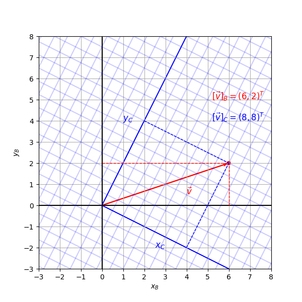
We now derive the coordinates of $\vec{v}$ relative to the basis $C$. To construct $[\vec{v}]_C$, we need the columns $[\vec{b_1}]_C$ and $[\vec{b_2}]_C$ of the change-of-coordinates matrix $\underset{C \leftarrow B}{\boldsymbol{P}}$.
These are obtained by expressing the basis vectors of $B$ as linear combinations of the basis vectors of $C$:

$$\begin{equation} x_1 \vec{c_1} + x_2 \vec{c_2} = \begin{pmatrix} 1 \\ 0 \end{pmatrix} = \vec{b_1} \end{equation}$$

and

$$\begin{equation} x_1 \vec{c_1} + x_2 \vec{c_2} = \begin{pmatrix} 0 \\ 1 \end{pmatrix} = \vec{b_2} \end{equation}$$

Row-reducing the augmented matrix of equation (1)_ yields

$$\begin{pmatrix} \begin{array}{cc|c} 0.5 & 0.25 & 1 \\ -0.25 & 0.5 & 0 \end{array} \end{pmatrix} \sim \begin{pmatrix}\begin{array}{cc|c} 1 & 0 & 1.6 \\ 0 & 1 & 0.8 \end{array}\end{pmatrix}$$

Similarly, equation (2) gives

$$\begin{pmatrix} \begin{array}{cc|c} 0.5 & 0.25 & 0 \\ -0.25 & 0.5 & 1 \end{array} \end{pmatrix} \sim \begin{pmatrix}\begin{array}{cc|c} 1 & 0 & -0.8 \\ 0 & 1 & 1.6 \end{array}\end{pmatrix}$$

Thus, the change-of-coordinates matrix $\underset{C \leftarrow B}{\boldsymbol{P}}$ is

$$\underset{C \leftarrow B}{\boldsymbol{P}} = \begin{pmatrix} 1.6 & -0.8 \\ 0.8 & 1.6 \end{pmatrix}$$

and we finally obtain

$$[\vec{v}]_C = \begin{bmatrix} [\vec{b_1}]_C \ [\vec{b_2}]_C \end{bmatrix} [\vec{v}]_B = \begin{pmatrix} 1.6 & -0.8 \\ 0.8 & 1.6 \end{pmatrix} \begin{pmatrix} 6 \\ 2 \end{pmatrix} = \begin{pmatrix} 8 \\ 8\end{pmatrix}$$

$\Box$

Application: View Transformation and Camera Space in OpenGL

Figure 2 shows a wireframe teapot mesh with a view camera targeted at it⁵. The interactive controls allow repositioning of the world and the view camera as well as the teapot, making it easy to visualize the different coordinate systems involved: The 3D world space versus the image produced by the camera⁶.

Figure 2: A wireframe teapot mesh rendered in a 3D scene, with a view camera targeting it. Use mouse controls to explore the scene interactively (open in new tab).

The abstracted camera also defines parameters for perspective projection, such as the field of view (fov) and the aspect ratio. However, for the purpose of constructing the view matrix, the most relevant parameters are the camera position, $\text{up}_{xyz}$ and $\text{eye}_{xyz}$, as they define the camera's position, its orientation and the view direction in world space. These parameters are used for constructing an orthonormal coordinate frame as we will show in the following sections.

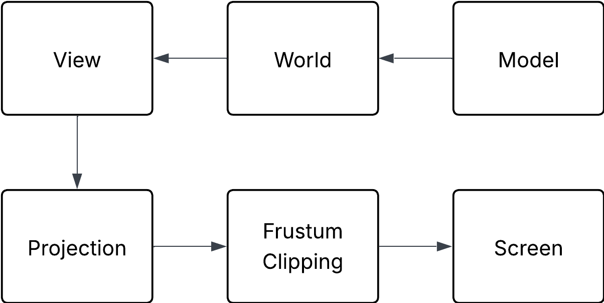
In the graphics pipeline [📖VB15, 232], transforming world coordinates $\vec{v}_\text{world} \in V_\text{world}$ to camera coordinates $\vec{v}_\text{cam} \in V_\text{cam}$ is typically the third step in the rasterization process, as illustrated in Figure 3.

^{Figure 3 An abstraction of the graphics pipeline. 'View' is responsible for mapping world-coordinate to view coordinates - that is, transforming points and vectors of the game world to an arbitrary camera, or point of view, most often determined through a player controlled camera. (Adapted from [Figure 7.1, 232, VB15]).}

Defining Eye and Target Position

The eye (or camera) position - labeled as Camera Position in Figure 2 - represents the location of the viewer in the world, also referred to as the vantage point.

As a position in $V_\text{world}$, it can either be represented as a point

$$\text{eye}_{xyz} \in \mathbb{R}^n$$

or equivalently as a vector from the origin

$$\vec{e} = \text{eye}_{xyz} - (0, 0, 0)$$

When moving freely in the world, the camera is directed at a point of interest (poi)

$$c \in \mathbb{R}^n$$

The pair $(\text{eye}_{xyz}, c)$ defines both the distance as well as the direction of the camera view. The forward vector $\vec{f}$, representing the viewing direction, is simply the difference between the point of interest and the camera position.

$$\vec{f} = c - \text{eye}_{xyz}$$

Constructing the Camera Basis

To construct a coordinate frame for the view space $V_\text{cam}$, a third component is required - the $\vec{up}$ - vector. This vector indicates the orientation of the camera's top - it can be thought of as the reference for the camera's vertical direction in view space. An intuitive analogy is a flight simulator: Rolling the airplane about its forward axis - the $z$-axis - effectively rotates the $\vec{up}$ vector and changes the percieved orientation of the game world.

In Figure 2, this up-direction is visualized by the small blue triangle on top of the view frustum.

Together with the forward vector $\vec{f}$, we can now construct an orthonormal camera frame for mapping points and vectors from $V_\text{world}$ to $V_\text{cam}$

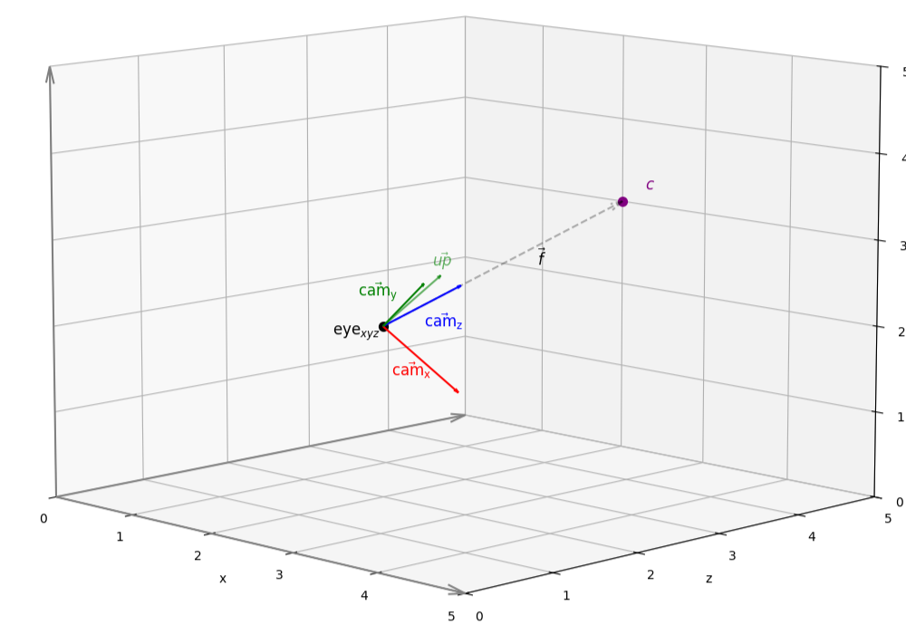
^{Figure 4 Starting from the viewer’s position, the vector toward the point of interest, and a given up‑vector, the camera’s coordinate system is constructed by orthonormalization. Note, that this illustration does not consider OpenGL's negative z-axis convention.}

Plot-Code (Python)

import matplotlib.pyplot as plt
import numpy as np
import math


fig = plt.figure(figsize=(10, 10))
ax = fig.add_subplot(projection='3d')

ax.set_xlim([0, 5])
ax.set_ylim([0, 5])
ax.set_zlim([0, 5])

ax.set_xlabel('x')
ax.set_ylabel('z')
ax.set_zlabel('y')

ax.quiver(0, 0, 0, 1, 0, 0, color='grey', length=5, arrow_length_ratio=0.04)
ax.quiver(0, 0, 0, 0, 1, 0, color='grey', length=5, arrow_length_ratio=0.04)
ax.quiver(0, 0, 0, 0, 0, 1, color='grey', length=5, arrow_length_ratio=0.04)

ax.view_init(elev=10, azim=-45)

camcol="black"
upcol="green"
poicol="purple"
camzcol="blue"
camxcol="red"
camycol="green"

eye = np.array([2, 2, 2])
poi = np.array([2, 5, 3])
up = np.array([1, 0, 1])
up_norm = up / np.linalg.norm(up)

camz = poi - eye
camz_norm = camz / np.linalg.norm(camz)

camx = np.linalg.cross(camz_norm, up_norm)
camx_norm = camx / np.linalg.norm(camx)

camy_norm = np.linalg.cross(camx_norm, camz_norm)
camy_norm = camy_norm / np.linalg.norm(camy_norm)

ax.text(*(poi - [0, -.3, -0.1]), r'$c$', color=poicol, fontsize=12, horizontalalignment='left')
ax.text(*(eye - [0, 0.6, 0.0]), r'$\text{eye}_{xyz}$', color=camcol, fontsize=12, horizontalalignment='left')

ax.scatter(*eye, color=camcol, s=50)
ax.scatter(*poi, color=poicol, s=50)

ax.quiver(*eye, *(camz), color='#000000', alpha=0.3,  arrow_length_ratio=0.05, linestyle="--")

ax.quiver(*eye, *(up_norm), color=upcol, alpha=0.6,  arrow_length_ratio=0.05)
ax.text(*(eye + [0, 0.6, 0.6]), r'$\vec{up}$', color=upcol, alpha=0.6, fontsize=12, horizontalalignment='left')

ax.quiver(*eye, *(camx_norm), color=camxcol,  arrow_length_ratio=0.05)
ax.text(*(eye + [0, 0.1, -0.6]), r'$\vec{\text{cam}}_\text{x}$', color=camxcol, fontsize=12, horizontalalignment='left')

ax.quiver(*eye, *(camz_norm), color=camzcol,  arrow_length_ratio=0.05)
ax.text(*(eye + [0, 0.5, -0.1]), r'$\vec{\text{cam}}_\text{z}$', color=camzcol, fontsize=12, horizontalalignment='left')

ax.text(*(eye + [0, 1.9, 0.4]), r'$\vec{f}$', fontsize=12, horizontalalignment='left')

ax.quiver(*eye, *(camy_norm), color=camycol,  arrow_length_ratio=0.05)
ax.text(*(eye + [0, -0.3, 0.4]), r'$\vec{\text{cam}}_\text{y}$', color=camycol, fontsize=12, horizontalalignment='left')

plt.subplots_adjust(left=0, right=1, top=1, bottom=0)
plt.show()

Although the OpenGL specifications explicitly state that

"OpenGL does not force left- or right-handedness on any of its coordinate systems."⁷

we adopt the widely accepted conventions found in standard textbooks and the OpenGL reference documentation itself ([📖SWH15]): These conventions assume a right-handed coordinate system in which the viewer looks down the negative $z$-axis, the positive $x$-axis extends to the right, and the positive $y$-axis points upward⁸.

Figure 4 shows a given up vector $\vec{up}$, the vantage point $\text{eye}_{xyz}$ as well as $c$ as the observed point. $\text{eye}_{xyz}$ and $c$ let us derive the forward vector $\vec{f}$. This vector - as well as subsequent vectors used in the following computations - is normalized.

We obtain $\vec{cam}_z$, which will serve as the $z$-axis of the required orthonormal basis of the camera space:

$$\frac{\text{eye}_{xyz}-c}{|\text{eye}_{xyz}-c|} = \vec{cam}_z$$

OpenGL z-axis conventions

Note that we subtract the point of interest $c$ from the camera position $\text{eye}_{xyz}$ to obtain a vector pointing in the opposite direction of the view vector in world space ($\text{eye}_{xyz}-c = - \vec{f}$). This inversion is necessary because the resulting camera space expects the view direction to be aligned with the negative $z$-axis⁹.

$\vec{cam}_z$ and $\vec{up}$ allow us to construct a perpendicular vector $\vec{cam}_x$, which becomes the $x$-axis of the camera frame:

$$\frac{\vec{up} \times \vec{cam}_z}{|\vec{up} \times \vec{cam}_z|} = \vec{cam}_x$$

To complete the basis, we compute $\vec{cam}_y$. While one might be tempted to use $\vec{up}$ directly, it is not guaranteed to be orthogonal to $\vec{f}$, since $\vec{f}$ is not a predefined axis but computed as the direction vector from $\text{eye}_{xyz}$ to $c$. Consequently, $\vec{up}$ may be slightly tilted toward or away from $\vec{f}$, as illustrated in Figure 4¹⁰.

$$\vec{cam}_z \times \vec{cam}_x = \vec{cam}_y$$

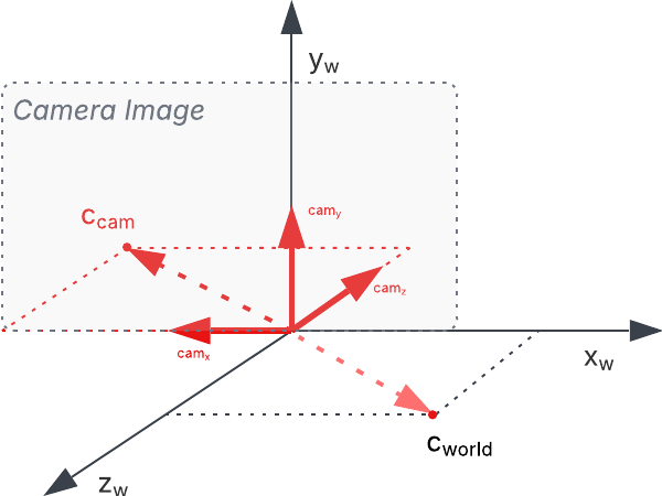
The derivation of the coordinate vector of point $c$ from world space to camera space is illustrated in Figure 5. In the figure, the camera is positioned behind the point of interest. As a result, the point - while located on the positive x-axis in world coordinates - is mapped onto the negative x-axis in the camera image.

^{Figure 5 Illustration of the orthonormalization process and the resulting camera image in a right-handed coordinate system. The bold lines represent the basis vectors of the camera coordinate frame. The point c is located on the positive x-axis in world space, but is projected onto the negative x-axis in the camera image due to the coordinate transformation.}

Transforming the World into Camera Space

Finally, we can construct the change-of-coordinates matrix $\underset{cam \leftarrow \text{world}}{\boldsymbol{P}}$.

Note that $V_\text{world}$ is represented by the standard basis $\varepsilon$. Therefore, the matrix

$$\begin{pmatrix} \vec{cam_x}_1 & \vec{cam_y}_1 & \vec{cam_z}_1 \\ \vec{cam_x}_2 & \vec{cam_y}_2 & \vec{cam_z}_2 \\ \vec{cam_x}_3 & \vec{cam_y}_3 & \vec{cam_z}_3 \end{pmatrix} = \underset{world \leftarrow \text{cam}}{\boldsymbol{P}}$$

contains the scalar components of the basis vectors of the camera frame expressed in world coordinate system. Its transpose yields the actual change-of-coordinates matrix from world to camera space:

$$\begin{pmatrix} \vec{cam_x}_1 & \vec{cam_x}_2 & \vec{cam_x}_3 \\ \vec{cam_y}_1 & \vec{cam_y}_2 & \vec{cam_y}_3 \\ \vec{cam_z}_1 & \vec{cam_z}_2 & \vec{cam_z}_3 \end{pmatrix} = \underset{cam \leftarrow \text{world}}{\boldsymbol{P}}$$

We now derive the translation vector $\vec{T}_{3 \times 1}$ used to complete the transformation.

By convention, the view camera is located at the origin $(0, 0, 0)$ and oriented to look down the negative $z$-axis. Objects that result in positive $z$-coordinates relative to the camera are typically clipped respectively culled from the final image.

To align the world such that the camera resides at the origin, we perform a translation by the negative eye position. This yields the following homogeneous translation matrix:

$$\begin{pmatrix} 1 & 0 & 0 & -\text{eye}_x \\ 0 & 1 & 0 & -\text{eye}_y \\ 0 & 0 & 1 & -\text{eye}_z \\ 0 & 0 & 0 & 1 \end{pmatrix}$$

With translation applied first, followed by rotation, we finally derive the complete lookAt-matrix

$$\boldsymbol{M}_{\text{lookAt}} = \begin{pmatrix} \underset{\text{cam} \leftarrow \text{world}}{\boldsymbol{P}} & \vec{T}_{3 \times 1} \\ 0 & 1\end{pmatrix}$$

as the product of rotation matrix and translation matrix¹¹

$$\begin{alignat*}{3} \boldsymbol{M}_{\text{lookAt}} &= \begin{pmatrix} \vec{cam_x}_1 & \vec{cam_x}_2 & \vec{cam_x}_3 & 0\\ \vec{cam_y}_1 & \vec{cam_y}_2 & \vec{cam_y}_3 & 0 \\ \vec{cam_z}_1 & \vec{cam_z}_2 & \vec{cam_z}_3 & 0 \\ 0 & 0 & 0 & 1 \\ \end{pmatrix} \begin{pmatrix} 1 & 0 & 0 & -\text{eye}_x \\ 0 & 1 & 0 & -\text{eye}_y \\ 0 & 0 & 1 & -\text{eye}_z \\ 0 & 0 & 0 & 1 \end{pmatrix}\\ \ \\ &= \begin{pmatrix} \vec{cam_x}_1 & \vec{cam_x}_2 & \vec{cam_x}_3 & -(\vec{cam_x} \cdot \vec{eye})\\ \vec{cam_y}_1 & \vec{cam_y}_2 & \vec{cam_y}_3 & -(\vec{cam_y} \cdot \vec{eye}) \\ \vec{cam_z}_1 & \vec{cam_z}_2 & \vec{cam_z}_3 & -(\vec{cam_z} \cdot \vec{eye}) \\ 0 & 0 & 0 & 1 \\ \end{pmatrix} \end{alignat*}$$

Derivation of the lookAt Matrix via Stepwise Inversion

(In the following, we implicitly assume that, whenever a $3\times 1$ vector $\vec{n}$ is multiplied by a $4\times 4$ matrix, $\vec{n}$ is interpreted as a homogeneous vector by appending a $1$ as its fourth component.)

Let $\vec{c_i}$ be the basis vectors of the camera space, expressed as coordinate vectors relative to the standard basis (that is, the basis of the world space).

The change-of-coordinates matrix $(\underset{\text{cam} \leftarrow \text{world}}{\boldsymbol{P}})^{-1} = \underset{\text{world} \leftarrow \text{cam}}{\boldsymbol{P}}$ is given by

$$\begin{pmatrix} c_{1_x} & c_{2_x} & c_{3_x} \\ c_{1_y} & c_{2_y} & c_{3_y} \\ c_{1_z} & c_{2_z} & c_{3_z} \end{pmatrix}$$

Mapping a vector $\vec{v}_\text{cam}$ from camera to world space gives

$$\vec{v}_\text{world} = \begin{pmatrix} c_{1_x} & c_{2_x} & c_{3_x} \\ c_{1_y} & c_{2_y} & c_{3_y} \\ c_{1_z} & c_{2_z} & c_{3_z} \end{pmatrix} \vec{v}_\text{cam}$$

However, to account for the position of the camera $\text{eye}_{xyz}$ - that is, the origin of the camera coordinate frame in world coordinates - we add $\vec{e}$ ($=\text{eye}_{xyz} - (0,0,0)$) to the rotated camera-space vector $\boldsymbol{R}(\vec{v}_\text{cam})$.

Hence, we obtain a transformation matrix

$$\vec{v}_\text{world} = \begin{pmatrix} c_{1_x} & c_{2_x} & c_{3_x} & e_x \\ c_{1_y} & c_{2_y} & c_{3_y} & e_y \\ c_{1_z} & c_{2_z} & c_{3_z} & e_z \\ 0 & 0 & 0 & 1 \end{pmatrix} \vec{v}_\text{cam}$$

How can we justify an inverse of this matrix through reasoning alone?

Since the original transformation from camera to world space consists of a rotation, followed by a translation, the inverse must reverse these steps - undo translation, then undo rotation:

$$\vec{v}_\text{cam} = (\underset{\text{world} \leftarrow \text{cam}}{\boldsymbol{P}})^{-1}\ \boldsymbol{T}(-\vec{e}) \ \vec{v}_\text{world}$$

where $(\underset{\text{world} \leftarrow \text{cam}}{\boldsymbol{P}})^{-1}$ is the inverse of $\underset{\text{cam} \leftarrow \text{world}}{\boldsymbol{P}}$, and $\boldsymbol{T}(-\vec{e})$ is a transformation matrix that adds $-\vec{e}$ component wise from the vector multiplied with it.

Obviously, due to associativity of matrix multiplications, we can compute the rotation-translation matrix first, which gives us

$$(\underset{\text{world} \leftarrow \text{cam}}{\boldsymbol{P}})^{-1}\ \boldsymbol{T}(-\vec{e}) = \begin{pmatrix} \underset{\text{cam} \leftarrow \text{world}}{\boldsymbol{P}} & \begin{matrix} -(\vec{c_1} \cdot \vec{e}) \\ -(\vec{c_2} \cdot \vec{e}) \\ -(\vec{c_3} \cdot \vec{e}) \end{matrix} \\ 0 & 1 \end{pmatrix}$$

Multiplying the vector $\vec{v}_\text{world}$ with this matrix will yield

$$\begin{alignat*}{3} (\underset{\text{world} \leftarrow \text{cam}}{\boldsymbol{P}})^{-1}\ \boldsymbol{T}(-\vec{e}) \ \vec{v}_\text{world} &= \begin{pmatrix} c_{1_x} & c_{1_y} & c_{1_z} & -(\vec{c_1} \cdot \vec{e}) \\ c_{2_x} & c_{2_y} & c_{2_z} & -(\vec{c_2} \cdot \vec{e}) \\ c_{3_x} & c_{3_y} & c_{3_z} & -(\vec{c_3} \cdot \vec{e})\\ 0 & 0 & 0 & 1 \end{pmatrix} \begin{pmatrix} {v_\text{world}}_x \\ {v_\text{world}}_y \\ {v_\text{world}}_z \\ 1 \end{pmatrix}\\ \\ &= \begin{pmatrix} c_{1_x} & c_{1_y} & c_{1_z} & -(\vec{c_1} \cdot \vec{e}) \\ c_{2_x} & c_{2_y} & c_{2_z} & -(\vec{c_2} \cdot \vec{e}) \\ c_{3_x} & c_{3_y} & c_{3_z} & -(\vec{c_3} \cdot \vec{e})\\ 0 & 0 & 0 & 1 \end{pmatrix}\begin{pmatrix} {v_\text{world}}_x \\ {v_\text{world}}_y \\ {v_\text{world}}_z \\ 1 \end{pmatrix}\\ \\ &= \begin{pmatrix} {v_\text{world}}_xc_{1_x} + {v_\text{world}}_yc_{1_y} + {v_\text{world}}_zc_{1_z} -(\vec{c_1} \cdot \vec{e}) \\ {v_\text{world}}_xc_{2_x} + {v_\text{world}}_yc_{2_y} + {v_\text{world}}_zc_{2_z} -(\vec{c_2} \cdot \vec{e}) \\ {v_\text{world}}_xc_{3_x} + {v_\text{world}}_yc_{3_y} + {v_\text{world}}_zc_{3_z} -(\vec{c_3} \cdot \vec{e})\\ 1 \end{pmatrix}\\ \\ &= \begin{pmatrix} ({v_\text{world}}_x - e_x)c_{1_x} + ({v_\text{world}}_y - e_y)c_{1_y} + ({v_\text{world}}_z- e_z)c_{1_z} \\ ({v_\text{world}}_x - e_x)c_{2_x} + ({v_\text{world}}_y - e_y)c_{2_y} + ({v_\text{world}}_z- e_z)c_{2_z} \\ ({v_\text{world}}_x - e_x)c_{3_x}+ ({v_\text{world}}_y - e_y)c_{3_y} + ({v_\text{world}}_z- e_z)c_{3_z}\\ 1 \end{pmatrix}\\ \\ &= \begin{pmatrix} (\vec{v}_\text{world} - \vec{e})\cdot \vec{c_1} \\ (\vec{v}_\text{world} - \vec{e})\cdot \vec{c_2} \\ (\vec{v}_\text{world} - \vec{e})\cdot \vec{c_3}\\ 1 \end{pmatrix}\\ \\ &= \vec{v}_\text{cam} \end{alignat*}$$

Here, $\vec{v}_\text{world} - \vec{e}$ yields a vector relative to the origin of the camera coordinate frame - the first step in the reverse operation (undo translation).

This vector is then projected onto the respective standard basis vectors, expressed in the camera basis ($[\vec{\varepsilon}_i]_c$), which form the rows of $(\underset{\text{world} \leftarrow \text{cam}}{\boldsymbol{P}})^{-1}$ (undo rotation).

The result is the same as if translation was applied first to $\vec{v}_\text{world}$ and then rotated:

$$\begin{alignat*}{3} \begin{pmatrix} (\vec{v}_\text{world} - \vec{e}) \cdot \vec{c_1} \\ (\vec{v}_\text{world} - \vec{e}) \cdot \vec{c_2} \\ (\vec{v}_\text{world} - \vec{e}) \cdot \vec{c_3}\\ 1 \end{pmatrix} &= \begin{pmatrix} c_{1_x} & c_{1_y} & c_{1_z} & 0 \\ c_{2_x} & c_{2_y} & c_{2_z} & 0 \\ c_{3_x} & c_{3_y} & c_{3_z} & 0\\ 0 & 0 & 0 & 1 \end{pmatrix} \begin{pmatrix} 1 & 0 & 0 & -e_x \\ 0 & 1 & 0 & -e_y \\ 0 & 0 & 1 & -e_z \\ 0 & 0 & 0 & 1 \end{pmatrix} \begin{pmatrix} {v_\text{world}}_x \\ {v_\text{world}}_y \\ {v_\text{world}}_z \\ 1 \end{pmatrix}\\ \\ &= \begin{pmatrix} c_{1_x} & c_{1_y} & c_{1_z} & 0 \\ c_{2_x} & c_{2_y} & c_{2_z} & 0 \\ c_{3_x} & c_{3_y} & c_{3_z} & 0\\ 0 & 0 & 0 & 1 \end{pmatrix} \begin{pmatrix} {v_\text{world}}_x -e_x \\ {v_\text{world}}_y -e_y \\ {v_\text{world}}_z -e_z \\ 1 \end{pmatrix}\\ \\ \end{alignat*}$$

---

Updates:

• 11.08.2025 Initial publication.

Footnotes

1. We intentionally emphasize the phrasing, as it contrasts with the more common convention of interpreting matrix columns as basis vectors. ↩

2. We follow Lay et al. [📖LLM21] with this notation. ↩

3. See [📖LLM21, 275] ↩

4. That is, the coordinate vector of $\vec{b_i}$ relative to $C$. ↩

5. Source code ↩

6. As this is a self‑contained scene observing itself, it resonates nicely with the spirit of Gödel, Escher, Bach. ↩

7. OpenGL 4.6 Core Profile, p.665 (retrieved 05.08.2025) ↩

8. "When the point of observation is located at the origin, as in perspective projection, objects drawn with positive z values are behind the observer." [📖SWH15, 83 ff] ↩

9. The illustration in Figure 4 shows a coordinate frame computed for a $+z$-convention. ↩

10. $|\vec{cam}_y| = 1$, since $|\vec{cam}_y| = |\vec{cam}_z \times \vec{cam}_x| = |\vec{cam}_z||\vec{cam}_x| \sin(\frac{\pi}{2}) = 1 \cdot 1 \cdot 1 = 1$ ↩

11. Note that the final column consist of dot products between the camera axes and the eye position vector $\text{eye}_{xyz}^{T}$ ↩

---

References

1. [LLM21]: Lay, David and Lay, Steven and McDonald, Judi: Linear Algebra and Its Applications Global Edition (2021), Pearson Deutschland [BibTeX]
2. [FH22]: Farin, Gerald E. and Hansford, Dianne L.: Practical Linear Algebra: A Geometry Toolbox (2022), CRC Press [BibTeX]
3. [VB15]: Van Verth, James M. and Bishop, Lars M.: Essential Mathematics for Games and Interactive Applications (2015), A. K. Peters, Ltd. [BibTeX]
4. [SWH15]: Sellers, Graham and Wright, Richard S. and Haemel, Nicholas: OpenGL Superbible: Comprehensive Tutorial and Reference (2015), Addison-Wesley Professional [BibTeX]